Keywords
Level set method (LSM); Image segmentation; Re-Initialization; Forward and backward diffusion (FAB); Single well potential; Double well potential; Triple well potential
Introduction
Stem cells are unique cells of the body in that they are unspecialized and have the ability to develop in to several different types of cells. Before injecting stem cells to the patients, first we have to analyse whether it is healthy or not. They are different from specialized cells, such as heart or blood cells and can replicate themselves. The analysis of stem cell includes segmentation, feature extraction, and pattern recognition. The preliminary process to find the growth rate of stem cell is segmentation. The main aim of this paper is to obtain the improved segmentation method to acquire the preliminary process in order to examine the growth rate of stem cells in future. Segmentation is one of the emphasise method in an image processing. It deals with sectionalisation of an image into multiple parts to recognize the objects like colour, texture, grey value, etc. and also image segmentation is the process of assigning a label to every pixel in an image such that pixels with the same label share certain characteristics. The success of image analysis depends on reliability of segmentation, but an accurate partitioning of an image is generally a very challenging problem. In image processing, there are many types of segmentation like thresholding, colour-based segmentation, transform method, texture based segmentation, partial differential equation-based method, etc. One of the partial differential equation-based techniques used here is called level set method. The level set method (LSM) is based on partial differential equations (PDE), i.e. active evaluation of the differences among neighbouring pixels to find object boundaries. Idyllically, the LSM will converge at the boundary of the object where the differences are the highest. LSM is used as a tool for numerical analysis of surfaces and shapes. The LSM method is mainly used for the image segmentation and it also find its application in image science.
History of Level Set Methods
In contemporary years, the level set methods find its application in many fields like computer vision, image processing, computer graphics, fluid dynamics computational geometry and optimization. The active contour based methods are used to deal about various image segmentation problems. There are two categories of active contour such as parametric active contour model [1] and geometric active contour model [2]. Parametric active contour models are as parametric curves described by Langrangian framework and geometric active contour models use curve evolution theory and denoted as level set function (LSF). The level set method was first introduced by Osher and Sethian [3] in 1987. The concept of level set is to symbolize the active contour as zero level set which is a higher dimensional function called level set function (LSF) and devise the motion of contour as the evolution of level set function. Level set methods are able to represent the contours of multifaceted topology and can handle the topological variations like splitting and merging in efficient way which cannot be done by parametric active contour model [1,4,5]. The changes in the shape and topology of contour can be expressed as curve and level set evolution. The evolution of curve [6] is expressed as
 (1)
(1)
Where β is the speed function that controls the speed of the contour and  is the inward normal vector of contour C(t). This C(t) can be described as zero level set function , C(t) ={(x, y) | (x, y, t) = 0} , here φ > 0 and φ < 0 represent the external (positive value) and internal (negative value) of the curve. The level set method is defined by the signed distance function (SDF) as
φ(x, y, t) = ±d((x, y),C(t)) (2)
Where d((x,y),C(t)) indicates the distance of a point on the plane to the curve. If the point locates inside the curve then the sign of the distance is negative or else it is positive. φ (x,y,t) satisfies  with the definition of SDF. The variation rate of φ (x,y,t) is uniform and it is useful for numerical calculation [7]. The inward normal vector in the curve evolution is given as
  where ∇ is the gradient operator. By using this, curve evolution in equation (1) is expressed in terms of partial differential equation as
 (3)
(3)
The above equation is mentioned as level set equation. During the evolution of contour due to the variation in velocity field of the image plane there occur irregularities of LSF, as a result the stability of the level set evolution is ruined and produce numerical errors. To get rid of this problem a numerical remedy called re-initialisation [8,9] is used to restore the regularity of LSF and maintain stable level set evolution. The concept of reinitialization is to stop the evolution instantly and remodelling the disgraced LSF as a signed distance function [9,10]. The reinitialisation method is mainly used to elucidate the evolution equation:
 (4)
(4)
Where (φ) is the LSF to be reinitialised and sign (φ) is the sign function. The solution for this equation will be signed distance function. The re-initialization method [10,11] is mostly used in many level set methods and other technique with fast marching algorithm [8]. Even though the re-initialization is able to maintain the regularity of LSF, it may erroneously move the zero level set to the unwanted position [8,9,12].
In variation level set method, there is no need for re-initialisation instead it uses a penalty term which will correct the deviation of the LSF from a signed distance function [13]. This penalty term will avoid the use of re-initialisation and also it is easy to get numerical scheme. However this causes an adverse side effect on the LSF in some points and affects the numerical accuracy.
To overcome the side effects, a new variation level set called distance regularization level set evolution (DRLSE) [14] uses distance regularization term and an external energy term. This method will avoid the re-initialisation by using the penalty term as potential function particularly double-well potential which will move gradient magnitude of the LSF. The regularity of the LSF is maintained by the forward and backward (FAB) diffusion [15]. Another method of DRLSE is proposed which uses an improved diffusion rate [16] to overcome the side effects in double well potential. In SRLSE [17] the distance regularization is applied to the image segmentation. DRLSE method is upgraded by providing an improved diffusion rate with triple well potential technique. This will avoid the side effects in DRLSE method and increases the accuracy and maintains the signed distance property [18].
System Method
System design describes block diagram for DRLSE with triple well potential. The time-lapse series of stem cell image is hired as input image and the distance regularisation method is enforced to segment the stem cell image. Here the triple-well potential is instigated to improve the segmentation process and the segmented output is compared with the preliminary single-well and double-well potential. The three potentials are explained in the down coming sections (Figure 1).
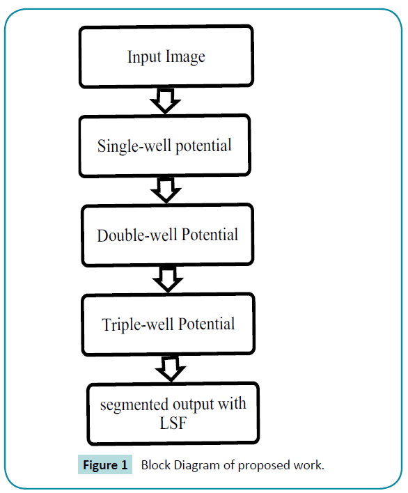
Figure 1: Block Diagram of proposed work.
Input image
The time-lapse image data of stem cells is chosen as an input image. Many experiments have been done for time lapse series [18] image segmentation; tracking and analysis of the morphological changes of cells are the challenging tasks in image processing. Stem cells are very powerful cells found in both humans and nonhuman animals. Stem cells are capable of dividing and renewing themselves for long periods. They are unspecialized cells which can give rise to specialized cell types (Figure 2).
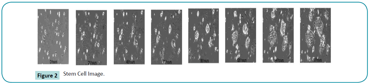
Figure 2: Stem Cell Image.
Single well potential
Segmentation is the process of partitioning the given image such that the required area of object can be obtained. There are many methods for the segmentation process and here it deals with distance regularization level set evolution [15].
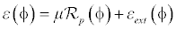
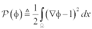
In level set methods [3], there is a problem of re-initialization. To overcome this problem a penalty term [14] is introduced in the distance regularization process. The level set energy function å(φ) on a domain Ω, is expressed as
 (5)
(5)
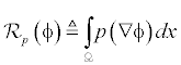
Where,  is the level set regularization termì is a constant and
  is the data term that depends on the image data. The level set regularization term is given by
 (6)
(6)
Where p:[0,∞] is a potential function which acts as the penalty term and it [14] is given as
 (7)
(7)
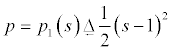
Which has one minimum point s=1 i.e. single well potential. The level set regularisation term with this potential is expressed as
 (8)
(8)
This is considered as the penalty term in our primary work [14,17]. This potential function maintains the signed distance property in the whole domain but it has some side effects in LSF φ at some positions.
Double well potential
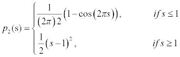
To avoid the side effects in the single well potential, Li [15] proposed a different variation method in which a new potential function p2(s) is proposed which is defined as
 (9)
(9)
There are two minimum points in this potential function p2(s) and they are s=0 and s=1. The first derivative for this potential is derived as
 (10)
(10)
This double well potential is able to maintain the signed distance property∇φ =1 but when∇φ < 0.5 , it approaches to 0 instead of 1 which will affect the regularity of the LSF.
Though the double-well potential has many advantages over preliminary work, it has certain drawbacks due to which this technique lags good results. If the initial LSF signed distance function  is smaller than 0.5 on all LSF domain, the DRLSE with dp2(s) fails to segment the object accurately because the distance regularization with dp2(s) loses the ability to regularize the LSF for
  . and makes to approach 0 instead of 1 which leads to undesirable side effects to the evolution.
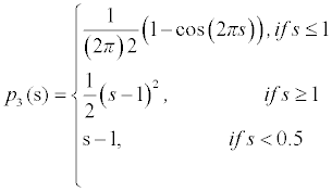
Triple-well potential for distance regularization
The energy function  is proposed as a penalty term in initial work in an effort to maintain the signed distance property in the entire domain. The consequent level set evolution for energy minimization has an undesirable side effect on the LSF φ in some circumstances. To avoid this side effect, a new potential function in the distance regularization term
  is introduced. This new potential function is aimed to maintain the signed distance property
  only in an area of the zero level set, while keeping the LSF constant with at locations far away from the zero level set.
To maintain such a profile of the LSF, the potential function must have minimum points at s=2, s=1 and s=0. Such a potential is a triple-well potential as it has three minimum points (wells). Using this triple-well potential p=p3 not only avoids the side effect that occurs in the case of p=p2, but also offers some tempting theoretical and arithmetical properties of the level set evolution.
This potential function maintains the signed distance function shape around the SDB (Signed Distance Band) with flat outside the band. The constant c0 will control the width of the SDB, because when the function φ becomes a signed distance function in the SDB, its values vary from -C0 to ∇φ =a1cross the band at a rate of ∇φ =1. This implies that the width of the SDB is approximately 2co. The potential function is derived as
The derivative of the above equation is given as
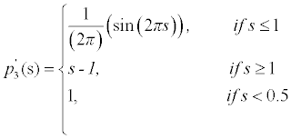
The above equation is used to find the regularization effect in the LSF. Here the three minimum points s=0, s=1, s=0.5 are used which is called as triple well potential. The condition is chosen as s-1 if s <0.5 since the gradient value s-1 will be 1 so that the edge can be segmented more clearly. By using this potential, LSF is maintained below 0.5 values of ∇φ . Thus the signed distance property is maintained in the desired locations.
Result and Analysis
The level set function of the desired region is obtained by implementation of distance regularisation effect as follows:
Step 1: Parameter setting
Step 2: Smooth image by Gaussian convolution
Step 3: Initialize LSF as binary step function
Step 4: Obtain the initial zero level contour
Step 5: Choose the potential function (single, double or triple)
Step 6: Start level set evolution
Step 7: Obtain the final zero level contour
Step 8: Display the final zero level contour in mesh to get final level set function.
The parameters like μ, α, λ are selected for the implementation. Then the image is smoothen by using the Gaussian convolution and then applied to the segmentation process. The initial level set function is in rectangular form. The potential function is chosen as either single-well  , which is good for regionbased model or double-well (eqn.8, which is good for both edge and region based models) or triple-well (eqn.10, which is also good for both edge and region based models). The accuracy of the triple-well potential is better when compared to the other two functions. This can be proved by using the precision and recall values.
Single-well potential analysis
In the single well potential, the potential function is used to choose the single minimum point. The binary step function is used as the initial function to stimulate the distance regularization effect.In the interior of the regions  and
and  the value of
  or the binary initial function. So, the single well potential has backward diffusion in the FAB diffusion with large diffusion rate. The strong backward diffusion significantly increases and cause oscillation in φ , which finally appears as periodic crests and dales in the converged LSF. The below (Figure 3a, b) shows the segmentation and their corresponding LSF it is clear that there is more peaks and valleys due to the oscillations.
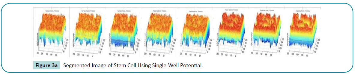
Figure 3a: Segmented Image of Stem Cell Using Single-Well Potential.
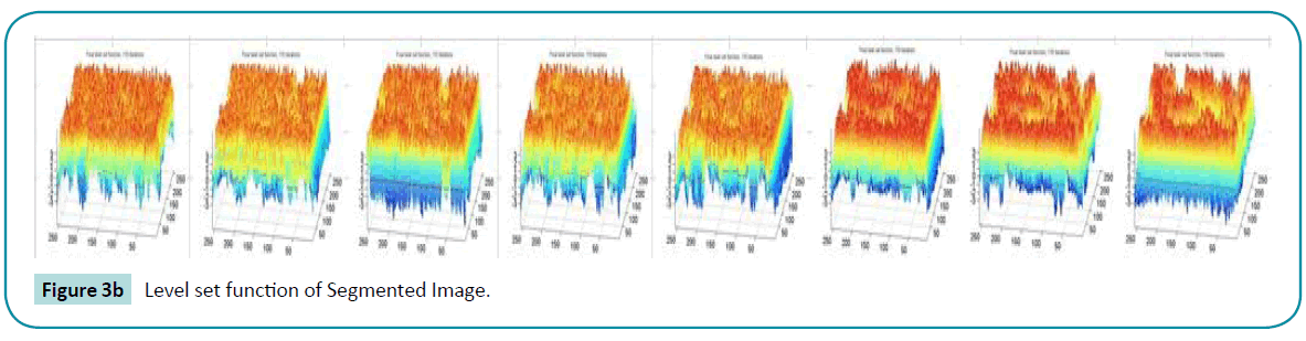
Figure 3b: Level set function of Segmented Image.
Double-well potential analysis
The diffusion rate is increased by using the double well potential in which the diffusion rate is maintained by using both the forward  and backward
  diffusion so that the signed distance property is maintained and the oscillations occurred in the diffusion rate with 1 p = p is eliminated. The segmented output of double-well is more accurate than the single-well potential. This can be clearly seen from the (Figure 4a, b) converged LSF given below.
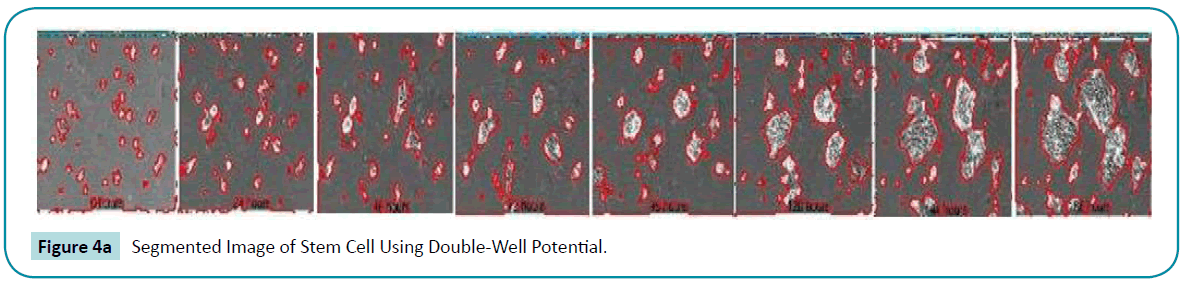
Figure 4a: Segmented Image of Stem Cell Using Double-Well Potential.
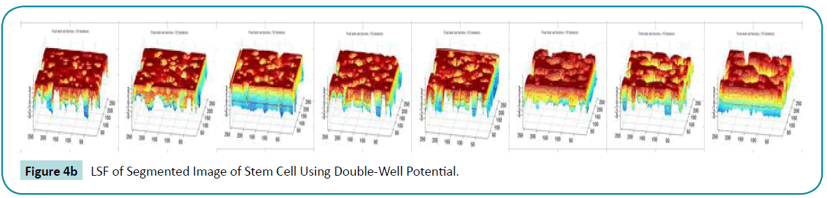
Figure 4b: LSF of Segmented Image of Stem Cell Using Double-Well Potential.
Triple-well potential analysis
In double-well potential, the signed distance function below 0.5 will decrease the value to zero but it should be one so that the signed distance property is not achieved. This problem is overcome by adding another potential called triple-well potential which will increase the diffusion rate by choosing another minimum point.
The accuracy is also increased and the number of iterations is reduced by increasing the time gap. The segmented output is so clear than the preliminary work this can be seen by the (Figure 5a, b).
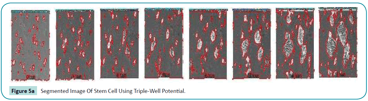
Figure 5a: Segmented Image Of Stem Cell Using Triple-Well Potential.
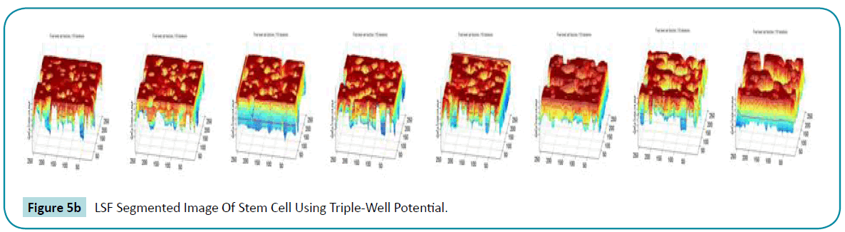
Figure 5b: LSF Segmented Image Of Stem Cell Using Triple-Well Potential.
The achievement of signed distance function in the signed distance band by using triple-well potential is clearly observed. The (Figure 6a) shows that the signed distance function is not attained even in the zero level set which will lead to the boundedness. By using the  , (Figure 6b) the signed distance function is achieved above the 0.5 value but failed in all domains and zero level set is also missing. (Figure 6c) represents the distance regularisation result of
  . The final LSF shows that the signed distance property is obtained in all domains by using three minimum points (wells) and also it possess the signed distance function shape in the signed distance band and flat outside the band which is controlled by the constant c0.
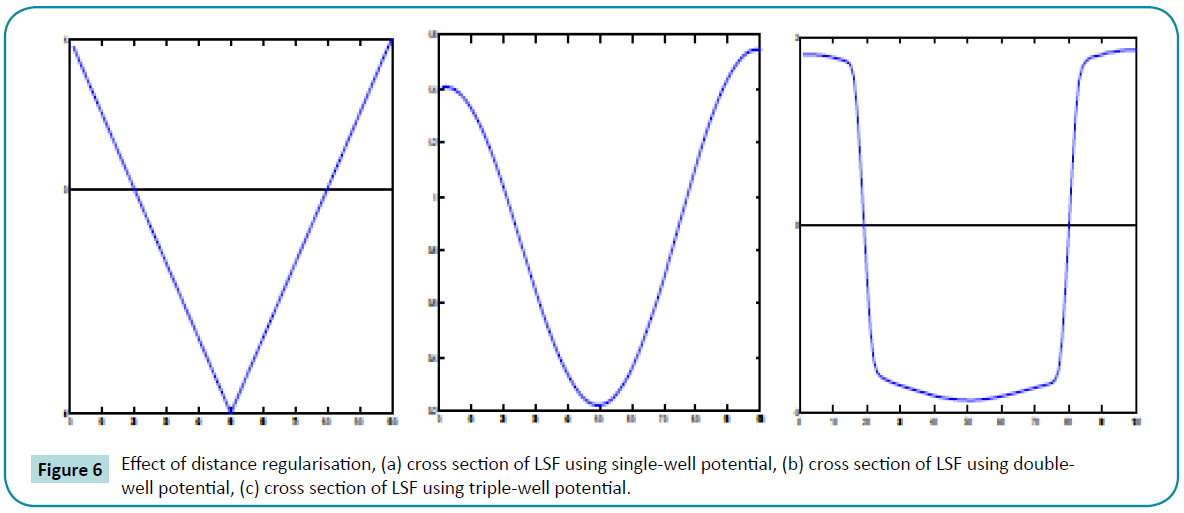
Figure 6: Effect of distance regularisation, (a) cross section of LSF using single-well potential, (b) cross section of LSF using doublewell potential, (c) cross section of LSF using triple-well potential.
Table 1 illustrates that the precision, recall and PSNR value of Triple well potential is gradually improved when compared to the single well and Double well. Because this method has the ability to maintain the signed distance property even when signed distance function is less than 0.5. And it disables the hurdles present in the previous technique. Due to its fast processing scheme there may be chances of over segmentation. Over segmentation can be avoided in future by controlling the direction of evolution in level set method by introducing balloon forces.
| Stem cell image |
Single well potential |
Double well potential |
Triple well potential |
| Hours |
Precision |
Recall |
PSNR |
Precision |
Recall |
PSNR |
Precision |
Recall |
PSNR |
| 0 |
76.62 |
93.71 |
32.14 |
80.42 |
94.71 |
38.3 |
81.98 |
96.25 |
45.15 |
| 24 |
81.62 |
9.27 |
34.18 |
82.42 |
94.27 |
40.15 |
83.98 |
95.81 |
46.40 |
| 48 |
83.62 |
92.84 |
35.15 |
84.42 |
93.84 |
40.94 |
85.98 |
95.38 |
46.91 |
| 72 |
85.62 |
9.41 |
35.73 |
86.42 |
93.41 |
41.40 |
87.98 |
94.95 |
47.19 |
| 96 |
87.62 |
91.97 |
36.12 |
88.42 |
92.97 |
41.70 |
89.98 |
94.51 |
47.37 |
| 120 |
89.62 |
91.54 |
36.40 |
90.42 |
92.54 |
41.91 |
91.98 |
94.08 |
47.49 |
| 144 |
91.62 |
91.11 |
3.61 |
92.42 |
92.11 |
42.07 |
93.98 |
93.65 |
47.58 |
| 168 |
9.62 |
90.68 |
36.78 |
94.42 |
91.68 |
42.19 |
95.98 |
93.22 |
47.45 |
Table 1: Performance analysis of single well, double well, triple well potential segmentation.
Monitoring cell confluence is valuable for optimization of cell culture parameters to provide efficient approach for detection of necrosis. Successful outcome of clinical studies are essential and next step is to implement innovative technological solution to deliver affordable clinical results to artificially reconstruct human tissue which has been previously damaged. The cells are extracted from the patients and they are grown under controlled in vitro condition in lab so that they can multiply and lead to grow with some addition of proteins or growth hormones to the culture medium and then implant to the patients. Using image processing on stem cell the future healthy parameters of the stem cell is analysed and viewed through results without any practical needs but in clinical approach it is quite difficult and also it needs more time for the process. Computerized analysis gives prior information for clinical approach to predict the healthiness of stem cell by its growth rate.
Conclusion
Thus the oscillations in distance regularization effect using singlewell potential and the side effects of double-well potential are overcome by using the triple-well potential. The segmentation of the time lapse series image of stem cell is done properly by using the triple-well potential distance regularization effect. The signed distance function is achieved in the zero crossing and the signed distance property is achieved in the signed distance band. The experimental analysis clears that the accuracy is increased by this method and the number of iterations also reduced. The level set function is regular and the signed distance property is also achieved using the triple-well potential. Hence the improved segmentation method achieves high precision, recall and PSNR values. This proposed technique pays way for the exploration of growth rate and healthiness of stem cells.
7217
References
- KassM, WitkinA,TerzopouloD(1987) “Snakes: Active ContourModels”.Int’l J Comp 1:321-331.
- Caselles V, Catte F, Coll T,Dibos F (1993) “A Geometric Model forActive Contours in Image Processing”.NumerMath 66: 1-31.
- Osher S, SethianJA(1988) “Fronts Propagating with Curvature Dependent Speed: Algorithms Based on Hamilton-JacobiFormulations”, J CompPhys 79: 12-49.
- ZhuSC, YuilleA (1996) “Region competition: Unifying snakes, regiongrowing, and Bayes/MDL for multiband image segmentation,” IEEETrans. Pattern Anal MachIntell 18: 884–900.
- XuC, PrinceJ(1998) “Snakes, shapes, and gradient vector flow, ”IEEE Trans. Image Process 7:359–369.
- KimiaBB, TannenbaumA, ZuckerS, (1995) “Shapes, Shocks, andDeformations I: the Components of Two-dimensional Shape and theReaction-diffusion Space”.Int’l J CompVis 15: 189-224.
- PengD, MerrimanB,OsherS, ZhaoH,Kang M (1999) “A PDE-basedFast Local Level Set Method”.J CompPhys155: 410-438.
- Sethian J(1999) Level Set Methods and Fast Marching Methods.Cambridge,U.K.: Cambridge Univ. Press.
- Osher S,Fedki R(2002) “Level Set Methods and Dynamic Implicit Surfaces”.New York: Springer-Verlag.
- Sussman M, Smereka P, OsherS (1994) “A level set approach for computingsolutions to incompressible two-phase flow.” J. ComputPhys114:146–159.
- Sussman M,Fatemi E (1999) “An efficient, interface-preserving level setre-distancing algorithm and its application to interfacial incompressiblefluid flow.” SIAM J SciComput20: 1165–1191.
- PengD, MerrimanB,OsherS, ZhaoH, KangM (1999) “A PDEbasedfast local level set method.” J ComputPhys 155: 410–438.
- LiC, Xu C, Gui C,FoxMD(2005) “Level Set Evolution withoutRe-initialization: A New Variational Formulation.” in Proc.IEEE ConfComputVis Pattern Recognit 1: 430–436.
- Li C, Xu C, Gui C, Fox MD (2010) “Distance Regularized Level SetEvolution and Its Application to Image Segmentation”.IEEE TransactionsImage Process 19: 3243–3253.
- GilboaG, SochenN,ZeeviY (2002)“Forward-and-backward diffusionprocesses for adaptive image enhancement and de-noising.” IEEETrans Image Process 11: 689–703.
- Weifeng Wu, Yuan Wu, Qian Huang (2012) “An Improved Distance Regularized Level Set Evolution without Re-initialization”IEEE fifthInternational Conference on Advanced Computational Intelligence(ICACI).
- KusumanchiAvinashkumar, SatyaSwathiBylapudi(2014) “ An Adaptive Technique for Regularized Level Set Evolution to Image Segmentation” IOSR Journal of Electronics and Communication Engineering 9.
- Maška M, Dan?k O, Garasa S, Rouzaut A, Muñoz-Barrutia A, Ortiz-de-Solorzano C et al.(2013) ”Segmentation and Shape Tracking of WholeFluorescent Cells Based on the Chan-Vese Model”.IEEE Trans Med Imaging 32: 995-1006