Keywords
Sudden cardiac arrest; Biomarker; Visibility graph; PSVG
Introduction
Sudden Cardiac Arrest (SCA) is a medical condition which occurs due to arrhythmia of the heart causing it to stop effectively pumping blood to the brain and body. The fallout is almost immediate as the victim succumbs to death often within an hour of the onset of the symptoms [1]. What makes SCA further dangerous is the fact that it can affect a person who appears to be healthy and is not suffering from a cardiac ailment [2]. However, people with some sort of coronary disorder are at a higher risk of SCA.
An implantable cardioverter defibrillator (ICD) is useful to restore normal heart beat in patients who have suffered ventricular tachycardia or fibrillation. Though ventricular fibrillation is the major cause of sudden cardiac arrests, there are other causes of SCA as well. Moreover, protection against sudden cardiac death by ICD implantation is invasive and expensive, and therefore target patients must be selected with very high predictive accuracy [1].
An entirely different approach towards early diagnosis of cardiac dysfunction has gained sufficient momentum which involves studying ECG signals of the heart using fractal analysis [3,4]. In the realm of SCA, fractal analysis of heart rate variability has been used to predict cardiac mortality [5]. In earlier works [6], using detrended fluctuation analysis technique, scaling exponents have been calculated to predict both arrhythmic mortality and the spontaneous onset of lifethreatening arrhythmias.
In this paper, we have applied the visibility graph technique [7,8] for a quantitative assessment of cardiac dysfunction in the event of SCA, and analysis of the observed results has led to some interesting finding, which might lead to a clinical tool for risk management. The paper is organized in the following manner. In section 2 the methods describing the analysis techniques in the context of chaos theory are summarized. Section 3 provides the description and source of the data as well as the analysis done on them and the summary of the results. The paper wraps up with a discussion and conclusion in section 4.
Method
Fractals and non-linear methods
Mandlebrot [9] introduced the concept of fractals. A fractal is a never ending pattern that repeats itself at different scales and exhibits a property called “self-similarity”. Fractals are observed all around us, with different scaling factors; from the tiny branching of our blood vessels and neurons to the branching of trees, lightning bolts, and river networks. Regardless of scale, these patterns are all formed by repeating a simple branching process. Any particular region of a fractal looks very similar to the entire region though not necessarily identical. The calculation of fractal dimension for measuring self-similarity is a significant area in the study of chaos. Following are the various methods proposed for measuring fractal dimension (FD):
• Spectral analysis
• Rescaled range analysis
• Fluctuation analysis (FA)
• Detrended fluctuation analysis (DFA)
• Wavelet transform modulus maxima (WTMM)
• Detrended moving average (DMA)
• Multi-fractal detrended fluctuation analysis (MF-DFA)
• The latest addition being PSVG or power of scale-freeness of a visibility graph.
Visibility graph
Lacasa et al. [8] formulated the visibility algorithm to convert a time series data into a graph called the visibility graph. The work further stated that fractal series convert into scale-free networks and its structure is related to the fractal nature (self-similarity) and complexity of the time series [8,10]. This methodology has been used for simulation of both artificial fractal series and real (small) series concerning Gait disease [7]. In this technique each node of the visibility graph represents a time sample of the time series, and an edge between two nodes shows the corresponding time samples that can view each other. The visibility graph algorithm maps time series X to its Visibility Graph. Let Xi be the ith point of the time series. Xm and Xn, the two vertices (nodes) of the graph, are connected via a bidirectional edge if and only if the below equation is valid.
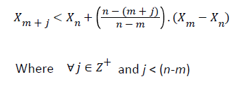
As shown in Figure 1, Xm and Xn can see each other, if the above condition is satisfied. With this logic two sequential points of the time series can always see each other hence all sequential nodes are connected together. The time series should be mapped to positive planes as the above algorithm is valid for positive values in the time series. The degree of a node in a graph is defined as the number of edges with the other nodes of the graph. P(k) or the degree distribution of the overall network formed from the time series is thereby the fraction of nodes with degree k in the network. Thus, if there are a total of n nodes in the network and nk of them have degree k, then P(k) = nk/n. Two quantities satisfy the power law when one quantity varies as a power of another. The scalefreeness property of a Visibility graph states that the degree distribution of its nodes satisfies the power law i.e. P(k) = k-λ, where λ is a constant and it is known as PSVG. PSVG, denoted by λ here, which is calculated as the gradient of log2P(k) vs log21/k, corresponds to the amount of complexity and fractal nature of the time series indicating Fractal Dimension FD of the signal [7,8]. Ahmadlou et al. applied the visibility graph algorithm to convert time series to graphs, while preserving the dynamic characteristics such as complexity [11]. It is also proved that there exists a linear relationship between the PSVG λ and the Hurst exponent H of the associated time series [7]. The visibility algorithm therefore provides an alternative method of computing the Hurst exponent. Also it has been shown, for example, that gait cycle (the stride interval in human walking rhythm) is a physiological signal that displays fractal dynamics and long-range correlations in healthy young adults. The algorithm of visibility graph predicts gait dynamics in slow pace, in perfect agreement with previous results based on the usual method of de-trended fluctuation analysis [7]. As the visibility graph is an algorithm that maps a time series into a graph, the methods of complex network analysis can also be applied to characterize a time series from a brand new viewpoint. Graph theory techniques can also provide an alternative method of quantifying long-range dependence and fractal nature in time series. Each pattern and behavior in a fractal time series is repeated frequently, in different scales, which has been proved by Ahmadlou et al. for a visibility graph, by calculating the PSVGs of a time series in multiple scales [12].
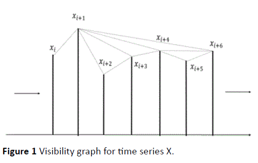
Figure 1 Visibility graph for time series X.
Using visibility graph algorithm we have converted the ECG time series data into visibility graphs at an interval of one minute across the time series. The present work is devoted to the calculation of PSVG values for each of the visibility graphs followed by a comparative analysis of PSVG values between diseased and normal subjects.
Results
Data
Data from two Physionet databases [13,14] have been used for analysis. The detailed description of the data is available on the website. The former database contains 23 complete Holter recordings for subjects experiencing sudden cardiac arrests while the latter contains 18 long-term ECG recordings of subjects having no significant arrhythmias. The naming conventions for the data followed in the subsequent texts of this paper are as per the website.
Analysis
The ECG data from diseased and normal subjects have been split in a manner such that each split spans approximately one minute of the ECG time series and consists of 10,000 data points being sampled across the span of a split.
With 10,000 data points the visibility graph of a split is constructed.
For each Visibility Graph, the value of P(k) is calculated for each of the values of k as described in Section 2. The variation of P(k) against k is found to satisfy the power law as shown in the Figure 2 (for a particular subject).
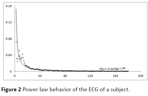
Figure 2 Power law behavior of the ECG of a subject.
The plot of log2P(k) vs log21/k is a straight line and, the gradient of the graph is the PSVG (Figure 3).
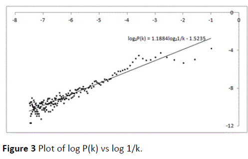
Figure 3 Plot of log P(k) vs log 1/k.
The mean PSVG i-th half-hour, j-th subject and standard deviation i-th half-hour, j-th subject are calculated for 30 consecutive splits (approximately 30 minutes) till the entire signal duration of the ECG is exhausted for each of the normal and affected subjects for each electrode. Thus, if the signal duration of a subject is T minutes, then the mean PSVG and SD are calculated for approximately T/30 splits for each of the normal and affected subjects for each electrode.
Once mean PSVG and SD calculation is done for all affected subjects for a particular electrode for each half an hour time interval of the entire signal duration of the ECG, the diseased mean PSVG i-th half-hour diseased is calculated across all affected subjects for each similar half hour interval for each electrode.
Similarly normal mean PSVG i-th half-hour normal and normal SD PSVG i-th half-hour normal are calculated across all normal subjects for each similar half hour interval for each electrode.
A plot of normal mean PSVG i-th half-hour normal and normal SD PSVG i-th half-hour normal is depicted in Figure 4 to show the trend of deviation of PSVG from the mean for the first 24 half hour intervals or first 12 hours.
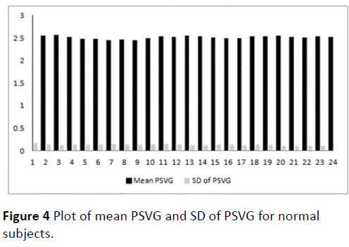
Figure 4 Plot of mean PSVG and SD of PSVG for normal subjects.
This is followed by a plot of PSVG i-th half-hour j-th diseased subject for a randomly selected diseased subject C42 for the first 24 half hour intervals or first 12 hours (Figure 5).
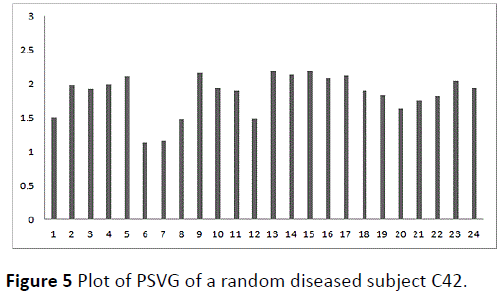
Figure 5 Plot of PSVG of a random diseased subject C42.
Next normal mean PSVG i-th half-hour normal and PSVG ith half-hour j-th diseased subject (for a randomly selected diseased subject C42) are plotted for the first 24 half hour intervals or first 12 hours as depicted in Figure 6.
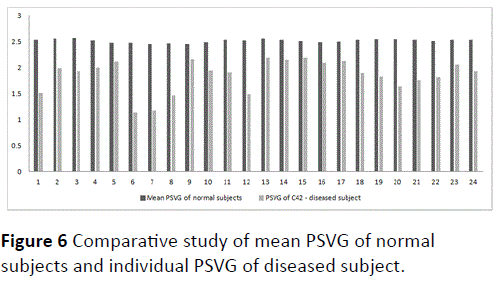
Figure 6 Comparative study of mean PSVG of normal subjects and individual PSVG of diseased subject.
Finally diseased mean PSVG i-th half-hour diseased and normal mean PSVG i-th half-hour normal are plotted for the first 24 half hour intervals or first 12 hours (Figure 7).
Observations
A number of interesting observations are obtained after the analysis as described below.
The plot of normal mean PSVG i-th half-hour normal and normal SD PSVG i-th half-hour normal in Figure 4 shows that deviations in PSVG values from the mean PSVG are significantly small in normal subjects. Hence it can be concluded that PSVG values of normal subjects hover around the mean. Also the mean PSVG of normal subjects remains steady over a span of 12 hours.
The plot of PSVG i-th half-hour j-th diseased subject for a randomly selected diseased subject C42 shows considerable fluctuations over a span of 12 hours as in Figure 5. Also the PSVG values of the diseased subject remain outside the range of normal mean PSVG i-th half-hour normal ± normal SD PSVG i-th halfhour normal as evident in Figure 6.
The comparative plot of values of mean PSVG for normal subjects and that of diseased subjects for 12 hours at an interval of ½ hour (Figure 7) reveals lower PSVG values for a diseased heart than that for a normal heart. The deviation of PSVG values of the affected patients from normal PSVG values remains within the range of 0.1 to 0.2 for the first 8 hours and henceforth becomes sharp with the PSVG shift going as high as 0.35 at a later point of time.
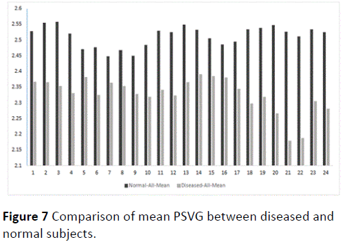
Figure 7 Comparison of mean PSVG between diseased and normal subjects.
Discussion
The higher values of PSVG indicate a better and stable functioning of the human heart [15]
Following parameters are obtained from the Visibility Network Graph analysis:
diseased mean PSVG i-th half-hour diseased
normal mean PSVG i-th half-hour normal
normal SD PSVG i-th half-hour normal
The plot (Figure 7) clearly shows that for diseased subjects mean PSVG is always less and this difference is statistically significant. Decrease in PSVG values is an indicator of dysfunction of the heart and the extent of deviation is an indicator of the degree of dysfunction.
The 3rd 1/2-hour probe gives an indication of a major dysfunction, which can be used to trigger an initial alarm. This gets pronounced at the 6th, 9th and 11th hours. There is a huge spike at the 11th hour indicating a serious medical condition.
This principle may be put to use for early detection of cardiac disorder in patients suffering from sudden cardiac arrest.
Conclusion
The fact that heart beat is chaotic enables us to analyze it using non-linear techniques e.g. visibility graph method. This analysis leads to formulation of certain parameters or biomarkers which may be used to detect abnormalities of the human heart sufficiently ahead of the time before it turns out to be fatal.
Initially, the software to compute and compare PSVG values may be used to detect onset of sudden cardiac arrest in hospitalized patients who are under ECG surveillance. As PSVG values start falling indicating a possible cardiac arrest, remedial action can be taken well before the dysfunction takes a fatal turn.
Eventually mobile apps may be prepared to compute the bio markers on a real time basis. The app will read data from an implanted loop recorder [16], compute PSVG and compare it with a benchmark PSVG preloaded for a healthy heart. Whenever the computed PSVG overshoots/ falls below the preloaded healthy PSVG by a pre-defined tolerance value, some audio visual markers will alert the individual of the impending cardiac disorder.
Acknowledgments
We thank the Department of Higher Education, Govt. of West Bengal, India for providing us the computational facilities to carry on this work.
13601
References
- Zipes DP, Wellens HJ (1998) Sudden cardiac death. Circulation 98: 2334-2351.
- George JJ, Mohammed EMS (2013) August. Heart disease diagnostic graphical user interface using fractal dimension. In Computing, Electrical and Electronics Engineering (ICCEEE). International Conference on IEEE 336-340.
- Beckers F, Verheyden B, Couckuyt KAA (2006) Fractal dimension in health and heart failure. Biomed Tech.
- Mäkikallio TH, Huikuri HV, Makikallio A, Sourander LB, Mitrani RD, et al. (2001) Prediction of sudden cardiac death by fractal analysis of heart rate variability in elderly subjects. J Am CollCardiol.
- Lombardi F, Makikallio TH, Myerburg RJ, Huikuri HV (2001) Sudden cardiac death: role of heart rate variability to identify patients at risk.Cardiovascular Research 50: 210-217.
- Lacasa L, Luque B, Luque J, Nuno JC (2009) The visibility graph: A new method for estimating the Hurst exponent of fractional Brownian motion. EPL EurophysicsLett 86: 30001.
- Lacasa L, Luque B, Ballesteros F, Luque J, Nuno JC (2008) From time series to complex networks: the visibility graph. ProcNatlAcad Sci 13: 4972-4975.
- Mandelbrot BB, Van Ness JW, van Ness JW (1968) Fractional Brownian Motions, Fractional Noises and Applications. SIAM Rev 10: 422-437.
- Dick OE (2012) Multifractal analysis of the psychorelaxation efficiency for the healthy and pathological human brain. Chaotic Model Simul 1: 219-227.
- Ahmadlou M, Adeli H, Adeli A (2010) New diagnostic EEG markers of the Alzheimer’s disease using visibility graph. J Neural Transm 117: 1099-1109.
- Ahmadlou M, Adeli H, Adeli A (2012) Improved visibility graph fractality with application for the diagnosis of Autism Spectrum Disorder. Phys A Stat Mech its Appl 391: 4720-4726.
- Peng CK, Mietus JE, Liu Y (1999) Exaggerated heart rate oscillations during two meditation techniques. Int J Cardiol 70: 101-107.
- Insertable loop recorders offer “the best opportunity” to diagnose unexplained syncope and abnormal heart rhythms. Cardiac Rhythm News.