Health Science Journal

Keywords

Data driven; Multiple myeloma; Statistical modeling

Introduction

Multiple Myeloma (MM), also known as Kahler disease, myelomatosis, and plasma cell myeloma is a type of cancer that starts from a malignant plasma cell (specifically the white blood cell) [1]. In the human body, the plasma cell produces antibodies as part of the human immune system that helps fight against germs and harmful substances. Myeloma is caused by the plasma cell becoming abnormal called the myeloma cell. With time, the myeloma cell accumulates in the bone marrow, where they crowd out healthy blood cells and may cause damage to the solid part of the bone. Multiple myeloma is therefore caused by the accumulation of the myeloma cells in the bones [2-8]. Figure 1 below shows the development of the myeloma cells [4-11].

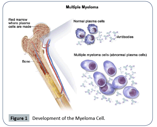
Figure 1: Development of the Myeloma Cell.

The abnormal plasma cells produce abnormal antibodies, which can cause kidney problems and overly thick blood [12]. The initial identified risk factors of MM include obesity, radiation exposure, family history, and certain chemicals [13-16]. Some recommended treatment for multiple myeloma is focused on decreasing the clonal plasma cell population and consequently decrease the symptoms of disease [17]. For patients under the age of 65, the preferred treatment is high-dose of chemotherapy, commonly with bortezomib-based regimens, and lenalidomidedexamethasone followed by autologous hematopoietic stem-cell transplantation (ASCT), that is, trans-plantation of a person’s own stem cells [18]. In 2017, a meta-analysis performed showed that post-ASCT maintenance therapy with lenalidomide enhanced progression-free survival and overall survival in persons at standard risk [19]. Whereas, in 2012, it was found from clinical trials that intermediate and high-risk disease patients benefit from a bortezomib-based maintenance regimen [20].

Statistics show that approximately 30,000 new patients are diagnosed with MM in the United States (U.S.) every year, becoming the second most common hematologic malignancy in the U.S. [21-24]. The Surveillance, Epidemiology and End Results (SEER) Cancer Institute reported in 2019 that MM constitutes 1.8% of all new cancer cases in the U.S. and ranked 14 among the list of cancer diseases [2]. They further projected that there will be an estimated number of 32,110 new cases of MM and an estimated 12,960 people will die of this disease. Those figures are staggering and overwhelming and cannot be overlooked. This is a rise compared with the estimated number of new MM cases of 24,050 reported in 2014 [3,6]. The established risk factors of MM are common among the age, black race, families with MM history, and being a male [2,7]. Reported earlier [2], 63.1% of all races and sexes of MM cases from 2012-2016 are aged 65 or greater.

Evidence about the risk factors or what typically causes MM remains scant. The existence of the myeloma plasma cell has not been quantified to be able to assess the contributing risk factors of MM. However, several risk factors have been identified to have some relation with the survival of patients with MM [9,10]. Most of these factors were identified at the time a patient was diagnosed with MM. Earlier studies [10,22,23] stated in their findings that hemoglobin, immunoglobulin type, extent and type of lesions, serum calcium, serum albumin, presence of Bence Jones protein, and performance status, at the diagnostic of MM are known to be essential in association with survival of patients with MM.

Some statistical analysis has been done on the survival of patients with MM given the event that a patient died or survived. Most of the research works done on MM has focused on how to improve the therapeutic strategy of MM. Brain et al. [9] used Kaplan and Meier to test whether there was a significant difference in the survival duration between the categories of risk factors based on the generalized Wilcoxon test and the log-rank test. They further used a non-linear Cox regression analysis to determined the combination of patients characteristics relative to survival duration. They identified a significant difference in the survival duration among patients based on performance status, cell mass and percentage labeling index, Nephrotic status, and Hemoglobin but no significant difference regarding patients age. Another statistical analysis by John M. Krall et al. [25] developed a set-up procedure for selecting variables associated with the survival times of patient with MM utilizing the data that we are using in the present study. They identified log blood urea nitrogen (BUN), hemoglobin, log percent plasma cells in bone marrow (BM) and Serum calcium to be associated with the survival of patients with multiple myeloma.

Durie and Salmon [22], developed a clinical staging system for MM based on the correlation of measured myeloma cell mass of 71 patients determined from the measurement of monoclonal immunoglobulin (M-component) synthesis and metabolism. They found a significant correlation of the measured myeloma cell burden with the extent of the bone lesion, hemoglobin level, serum calcium level, and M-component levels in serum and urine. However, serum creatinine/BUN had a strong correlation with the survival, and not the myeloma cell mass [26-31]. Their findings produced a clinical staging system based on 3 tumor cell mass indices, namely, low (0.6 × 1012 cells/sq m), intermediate (0.6−1.2 × 1012 cells/sq m) and high (>1.2 × 1012 cells/sq m). Merlini et al. [32], proposed a new improved clinical staging system for the survival of MM based on the analysis of 123 treated patients. They found serum calcium, % bone myeloma plasma cell (% BMPC) and serum creatinine/BUN to be strongly associated with the survival of IgG myeloma stage; hemoglobin, serum calcium, and M-component to be strongly associated with the survival of IgA myeloma stage; and creatinine/BUN, % BMPC and serum calcium to be strongly associated with the survival of BJ myeloma stage. Durie, et al. [9] proposed a pretreatment tumor mass, cell kinetics, and prognosis in MM of 150 patients base on the % labeling index (LI%) and DNA synthesizing cells (S). The findings of LI% <1% was associated with long survival, LI% > 3% in high cell mass patients with high S had a very poor prognosis.

In the present study, we developed a real data-driven statistical model of the significant attributable risk factors of survival time of patients diagnosed with multiple myeloma. The clinical trial that was conducted consisted of 65 patients who were diagnosed with MM. However, our study concentrated on 48 of the patients that we have death times (survival times) from diagnosis. The remaining 17 patients, we did not have information about their death times, so they were excluded from our analysis and modeling. Because of the low amount of the data, we did the modeling utilizing the 48 pieces of information. The data was filtered to fulfill all the modeling assumptions. After the development of the statistical model, we used the bootstrapping, resampling method to increase the amount of information, and then improved the accuracy of our statistical model. We identified the significant risk factors, and interaction contributing to the survival time of MM. The significant risk factors including the interaction identified were ranked based on the percentage of contribution to the death of MM patients, using the coefficient of determination (R2) of the survival times. The quality and accuracy of the proposed model was assessed based on the R2 along with the R2 adjusted statistic, the Akaike information criterion (AIC) of model selection, the prediction error sum of squares (PRESS), the root mean square error (RMSE), the variance inflation factor (VIF), the residual analysis, and the prediction accuracy (the correlation of the actual and predicted survival times based on 80% training set and 20% testing set).

Method

Data description

The data used in this research is from West Virginia University Medical Center provided by Harley [25,26]. Originally, the data constituted survival times of 72 multiple myelomas (MM) patients diagnosed and treated with alkylating agents [25]. 65 out of 72 patients provided complete data for 16 concomitant variables (risk factor) whiles the remaining 7 were eliminated due to missing data in at least one of the 16 risk factors. Given that a patient is diagnosed with myeloma, the 16 risk factors were recorded and the time up to which the patient survived the disease was also recorded (called the survival time from diagnosis to the nearest month). Of the 65 patients, 48 and 17 were dead and alive, respectively. In the present research, we utilized the complete data of the 48 patients death times for our analysis and modeling. The survival time of patients is the response variable with the information of the 16 the risk factors listed below. Thus, we have one continuous response variable, 11 continuous risk factors, and 5 categorical risk factors. The detailed description of the response variable and the 16 risk factors are given in Table 1 below.

Table 1 Variable Recorded for Multiple Myeloma Patients (Risk Factors).

Symbol	Variable Name
t	Survival time from diagnosis to nearest month +1
X1	Log blood urea nitrogen (BUN)/serum creatinine at diagnosis
X2	Hemoglobin at diagnosis
X3	Platelets at diagnosis 0 abnormal, 1 normal
X4	Infections at diagnosis 0 none, 1 present
X5	Age at diagnosis (complete years)
X6	Gender 1 male, 2 female
X7	Log white blood cell (WBC) at diagnosis
X8	Fractures  at diagnosis 0   none, 1  present
X9	Log %BM at diagnosis (log % plasma cells in bone marrow)
X10	% Lymphocytes in peripheral blood at diagnosis
X11	% Myeloid cells in peripheral blood at diagnosis
X12	Proteinuria at diagnosis
X13	Bence Jone protein in urine at diagnosis 1 present, 2 none
X14	Total serum protein at diagnosis
X15	Serum globin (gm%) at diagnosis
X16	Serum calcium (mgm%) at diagnosis

Before we proceeded to develop the statistical modeling of the survival times of patients diagnosed with multiple myeloma, we wanted to know whether there is a difference in the survival times with respect to gender, i.e. Male and Female. Given that we have a small data of only 48 patients, we used the log-rank test [27,28] from Kaplan Meier non-parametric test and compare the differences in survival times of male and female. From Figure 2 below, the log-rank test resulted in a large p-value=0.45, indicating a failure to reject the null hypothesis that there is no difference with respect to gender. This is a good justification to proceed with the building of the statistical model for the survival time of patients with MM since there is no bias concerning gender.

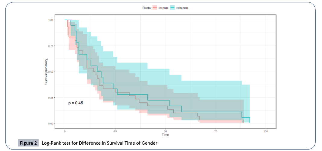
Figure 2: Log-Rank test for Difference in Survival Time of Gender.

Statistical modeling

We develop a statistical model for the survival times (death times) of the 48 patients diagnosed and died of multiple myeloma. In the building of the statistical model for multivariate linear regression, the following assumptions must be satisfied:

Linearity

There should be a linear relationship between the response variable t (survival time) and the risk factors including interactions. This is expressed as

(1)

where the response variable ti=(t1,...,tn)T, α=(1,...,1)T is the model intercept parameter, β=(β1,...,βk)T is the coefficient parameter of the attributable risk factors Xi’s, ρij is the coefficient parameter of interaction between ith and jth attributable risk factors, εi=(ε1,...,εn)T represents the model residual error term, and k=16 and n=48 is the number of attributable risk factors and the sample size, respectively. Linearity was assessed using the matrix of scatter plots and correlation between the response and the continuous risk factors.

Multivariate normality

The errors should follow Gaussian normal probability distribution with zero mean and standard deviation of one, ε ∼ N (0,1) as n → ∞. This was tested using the normal probability Q-Q plot and was verified using a formal test of normality i.e. the Shapiro Wilk’s test with the null hypothesis H0, that the residuals errors follow the normal probability distribution.

Homoscedasticity

The residual errors should have constant variance, var (εi)=σ2. We verify this by observing the plot of residuals versus fitted values; no pattern implies errors have constant variance. We then supported it with a formal test of non-constant variance with the null hypothesis H0, that the variance of the errors is constant.

None or very minimum multicollinearity

The risk factors should not be highly correlated. Usually, a correlation coefficient of r ≥ 0.9 indicates a very high correlation. A formal test for multicollinearity is using the variance inflation factor implies the presence of multicollinearity.

No autocorrelation

Residual errors are independent and uncorrelated, εi ∼ i.i.d / N (0, σ2). We checked this using a formal test of autocorrelation, i.e. Durbin Watson test with null hypothesis H0, that there is no autocorrelation.

We started by visually inspecting the matrix of scatter plot to assess the linear relationship between the response variable t and the continuous risk factor Xi. As shown in Figure 3, there is a weak linear relationship between the response variable t, and all the continuous risk factors given that the highest correlation coefficient is r=0.31, which is with X1. The distribution of the survival times t is right-skewed as it follows the three-parameter log-normal probability distribution (from the parametric analysis). We can see that some of the risk factors have skewed shaped distributions (a possible influence of outliers or extreme values). However, we continued to fit a model of the response variable as a function of the 16 attributable risk factors resulting in a coefficient of determination (R2)of 0.48 (48%); this cannot be considered a good model given that there are discrepancies associated with the data such as skewness or kurtosis [29-33]. However, fitting the first model to the original data allow us to check for other model assumptions.

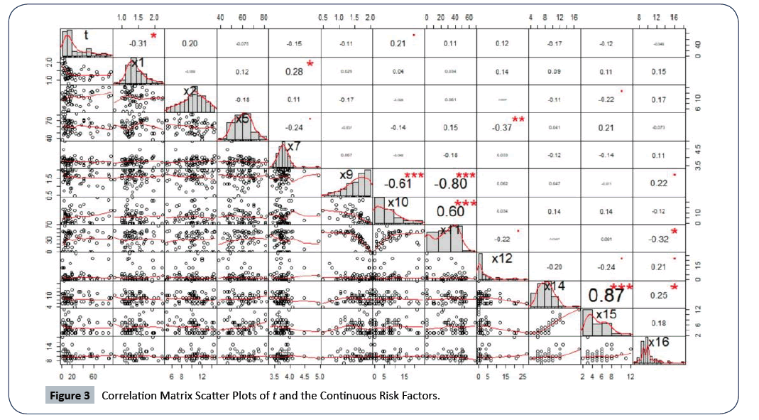
Figure 3: Correlation Matrix Scatter Plots of t and the Continuous Risk Factors.

In Figure 4, we plotted the Q-Q plot of residuals of the model built from the original data to assess the multivariate normal probability distribution. There is evidence of violation from normality as shown by the skewed ends of the Q-Q plot. A formal test for normal distribution using the Shapiro Wilk’s normality test resulted in a p-value=8.632e−03, which is an indication of lack of the normal probability distribution. This implies that the survival time t of patients with multiple myeloma does not follow the Gaussian probability distribution.

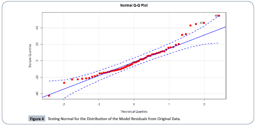
Figure 4: Testing Normal for the Distribution of the Model Residuals from Original Data.

Given that there is weak linear relationship and no multivariate normality, we applied log transformation to the response variable t and the skewed risk factors X10, X12, X14 and X16. Log transformation stabilizes the variance and suppresses the impact of outliers or extreme values in the data [29]. The transformations are giving by the expressions below:

(2)

and

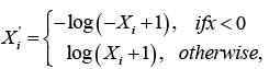
Where X i denotes the transformed risk factor of Xi. After the variable transformations, we proceeded to fit the full model for the survival times t as a function of the 16 risk factors and all twoway interactions between them. We then utilized the backward elimination procedure for model selection to find the attributable risk factors and the interaction(s) that significantly contributes to the survival time t. The backward elimination model selection technique is often used because it provides less bias mean square error (MSE) values and turns to prevents overfitting of the model, which is essential for the prediction performance of the model. Using this method of model selection, we selected the best model with the least Akaike information criterion (AIC=2ln(L) + 2k, where L is the value of the maximum likelihood function of the model and k represents the estimated model parameters) [27]. AIC gives an estimation of the relative amount of information missing in the model; hence, the smaller the AIC value the better the quality of the model. Therefore, given the model selection method and criterion of choice of a good model, the best-proposed model with R2=0.8741 which includes all the attributable risk factors and interaction that significantly contributes to the survival time of patients with multiple myeloma is given by

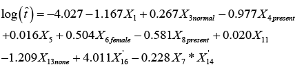(3)

Thus, there are nine attributable risk factors, namely, Bence Jone protein in urine, blood urea nitrogen (BUN)/serum creatinine, infections, % myeloid cells in peripheral blood, fractures, serum calcium, gender, platelets and age, and one interaction term, namely, white blood cells and total serum protein that significantly contribute to the survival of MM patients. The following remaining five risk factors do not contribute to the survival time of MM patients at diagnostic: hemoglobin, plasma cells in bone marrow, lymphocytes in peripheral blood, proteinuria and serum-globin (gm%). Because the estimated survival time t' and the attributable risk factors ' i X from equation (3) are based on the log-transform data from equation (2), we utilized the anti-logarithmic to transform back to the original values. The backward transformation of the attributable risk factors X14 and X16 can be expressed as

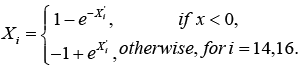(4)

To use the above proposed model given by equation (3), we first take the anti-logarithmic of the log transform attributable risk factors into the original values, given in equation (4). We then take the anti-logarithmic of the entire model in equation (3) to arrive at the actual estimate of the survival time of an MM patient.

Now, given the above-proposed model of survival time t of patients diagnosed with multiple myeloma, one may ask how useful can this model be? If a new patient is diagnosed with multiple myeloma, then given the values of the significant attributable risk factors identified in equation (3), we can use our proposed statistical model to accurately estimate the survival time of that patient.

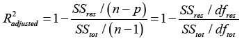
How accurate are the results/usefulness that we obtain in using the proposed nonlinear statistical model? We answer this question using the coefficient of determination statistic, R2 along with . The R2 is generally used to measure the goodness-of-fit of a statistical model. It estimates the proportion of variation in the response variable explained by the model attributable risk factors [30,31]. The higher the R2 statistic the better the goodness-of-fit of a statistical model. In general, the R2 is defined by

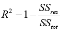(5)

Where and ti are the survival times, is the estimated survival time in equation (4). SSreg is the regression sum of squares representing the variation explained by the proposed model, SSres is the residual sum of squares representing the variation in the proposed model left unexplained and SStot is called the total sum of squares is the proportional to the sample variance, and equals to the sum of SSreg and SSres. Generally, the R2 has the problem of increasing by increasing the number of parameters or predictors in the model. Therefore, it is recommended that we estimate the R2 along with the R2 adjusted to adjust for the degrees of freedom of the model, and is given by

(6)

Our proposed statistical model given in equation (3) resulted in an R2 of 87.41% of 87.41%. This means the proposed model explains 87.41% variation in the response variable (i.e. the survival time of MM patients), a very good quality model.

Bootstrapping with the proposed statistical regression model

To further improve the efficiency of the proposed statistical model, we utilized the bootstrapping resampling method that due to Efron (1979). Bootstrapping is a general approach to statistical inference that allows assigning measures of accuracy (defined in terms of bias, variance, confidence intervals, prediction error or some other such measure) to sample estimates based on building a sampling distribution for a statistic by resampling from the actual data that we analyzed in the present study [34]. We applied the bootstrap sampling to resampled with replacement the data used to build the proposed analytical model given by equation (3); increasing the sample size by 300. This asymptotically increased the level of significance of the coefficient estimates, making them equally highly significant, and increased both the R2 and R2adjusted to 91.16% and 90.85%, respectively. The modified version of the model in equation (3) based on the bootstrapping resampling method is given by

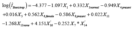(7)

Validation of the Proposed Statistical Model

Before validating the proposed model, we need to be sure that all assumptions that underline our proposed model are satisfied. We tested for linearity by showing the linearity plot (sometimes referred to the partial residual plot) of the response variable and the significant attributable risk factors as shown in Figure 5, below. We can see that there is a well-established linear relationship between the response variable and the continuous attributable risk factors (shown by the blue and pink lines). Therefore, the linearity assumption which was initially a problem we encountered has been rectified in our final proposed statistical model.

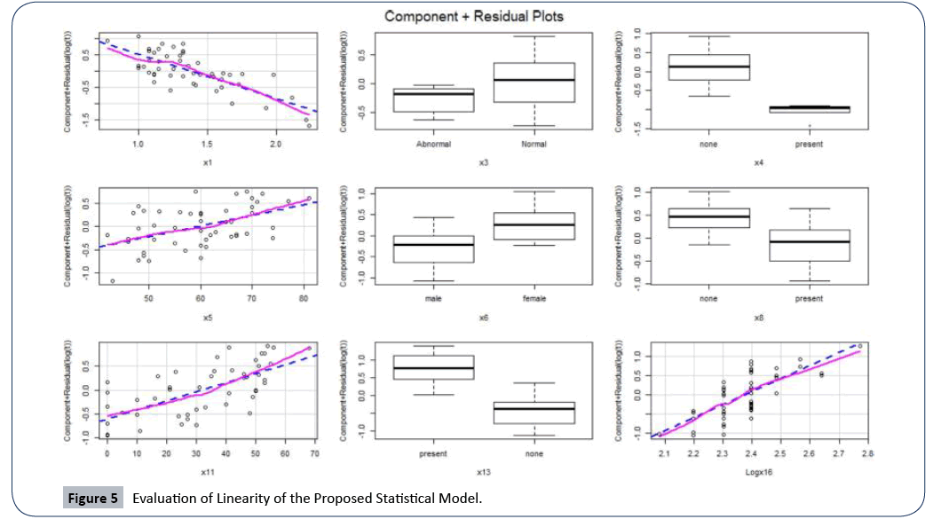
Figure 5: Evaluation of Linearity of the Proposed Statistical Model.

To verify that the proposed statistical model satisfies multivariate normal probability distribution assumption, we used the normal Q-Q plot shown by Figure 6. We see that the residuals are normally distributed with no major outlier and all the points in the plot fall within the 95% confidence bound. The evidence of normality is supported by the Shapiro Wilk’s test of the normal probability distribution (a formal test), given by a high p-value of 0.818. The plot of the distribution of studentized residuals in the second panel of Figure 6, is further evidence that the proposed model’s normality assumption is valid.

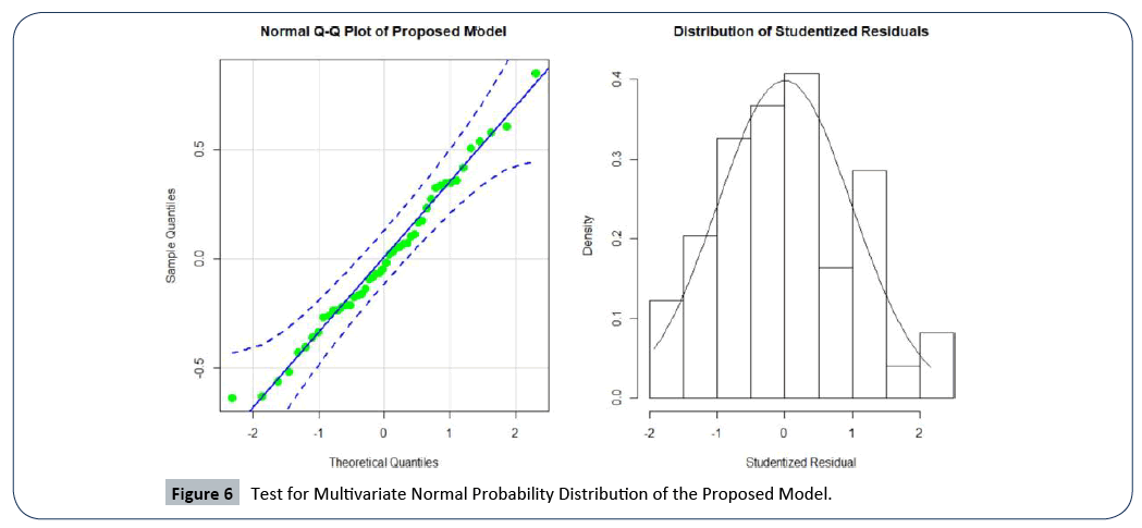
Figure 6: Test for Multivariate Normal Probability Distribution of the Proposed Model.

We performed residual analysis to assess the model residuals and constant variance. Figure 7, depicts the residual plot of the proposed model. Thus, we can conclude that there is no problem of homoscedasticity.

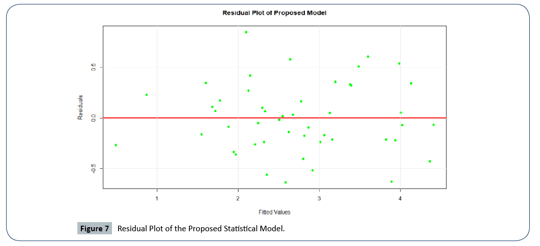
Figure 7: Residual Plot of the Proposed Statistical Model.

Our proposed statistical model perfectly satisfies the assumption of constant variance, indicated by the randomly scattered points about the zero line with no major outliers. A formal test for homoscedasticity revealed a p-value of 0.506, strongly supports that homoscedasticity of our proposed model is valid.

The mean absolute value of the residuals,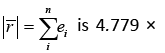 e−2, close to zero and the variance 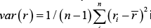is 0.636. The proposed statistical model has a very small root mean square error .

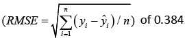Multicollinearity is a major problem in statistical modeling which must be addressed. It can distort the precision of the estimated coefficients leading to overfitting and misinterpretation on the results of the model. All the estimates of the parameters in our proposed model have a very small variance inflation factor VIF < 3 indicating that there is no problem of multicollinearity. Also, we expect the model residuals to be independent and uncorrelated. We tested for the presence of autocorrelation among errors in the proposed model using the Durbin Watson of testing the null hypothesis H0, no autocorrelation is present. Accepting the hypothesis with a large p-value of 0.624 indicated that there is no autocorrelation among residuals in our proposed model.

To validate the prediction accuracy of our proposed statistical model, we trained 80% of the data to build our model and tested on the remaining 20% test data. The prediction of the original model and the trained model using the test data is given in Table 2. We checked the accuracy of the predictions by finding the correlation coefficient r and the corresponding R2 (square of r) between the actual and the predicted values. This resulted in R2 of 0.943, a very high prediction accuracy. The comparison of the logarithmic survival times with the two models (i.e. model developed using all the 48 patients and the 80% trained model) prediction on the test data resulted in R2 of 0.943 and 0.930, respectively, attesting to the high prediction accuracy of our proposed model.

Table 2 Comparison of Prediction of the Survival Time of Multiple Myeloma.

Log(t)	Original Model	Trained Model
0.2231	0.4917	0.6379
1.0986	0.8676	1.3378
1.6094	1.9708	2.3358
1.9459	1.5979	1.1624
2.3979	2.1245	2.0809
2.7726	3.0083	2.9017
3.1781	3.1269	2.6158
3.7136	3.39	3.1649
3.9889	3.4851	3.2839
1.3863	1.5493	2.1449

Ranking of the contribution of attributes/ risk factors of the survival times of multiple myeloma

In this section, we rank the individual significant risk factors and the interaction based on their contribution to the survival time of MM patients using the percentage of R2. Table 3 shows the rank of each of the identified significant risk factors and the interaction term. Bence Jone protein in urine is ranked first, followed by blood urea nitrogen (BUN), the interaction term is ranked eighth, and age has the least contribution to the survival time of patients diagnosed with multiple myeloma (MM) among the significant attributable risk factors. A detailed discussion of the rankings will continue in the next section.

Table 3 Rank of Contribution of Attributing Risk Factors to Survival Time.

Rank	variable	Description	R2	% Contribution
1	X13	Bence Jone protein in urine at diagnosis 1-present, 2-none	0.2672	30.57
2	X1	Log BUN at diagnosis	0.2052	23.48
3	X4	Infections at diagnosis 0 none, 1 present	0.0949	10.86
4	X11	% Myeloid cells in peripheral blood at diagnosis	0.089	10.18
5	X'16	Serum calcium (mgm%) at diagnosis	0.0661	7.56
6	X8	Fractures at diagnosis 0 none, 1 present	0.0613	7.01
7	X7 & X'14	Log WBC at diagnosis and Total serum protein at diagnosis	0.0379	4.34
8	X6	Gender 1 male, 2 female	0.0329	3.76
9	X3	Platelets at diagnosis 0 abnormal, 1 normal	0.011	1.26
10	X5	Age at diagnosis (complete years)	0.0086	0.98
Total			0.8741	100

Discussion

The evaluation of the survival time of patients diagnosed with MM is an essential prerequisite for improving the prognosis and therapeutic/treatment strategy of multiple myeloma. The present study was designed to find a real data driven statistical model that accurately predicts the survival time from diagnosis to the nearest month of multiple myeloma patients deaths. In the present study we accomplished the following:

• We identified the significant attributable risk factors.

• We identified the significant interactions among the risk factors.

• We determined the percentage of contributions of each identified risk factor and interaction that causes the death of the patients.

It was important to assess whether there is a difference in the survival times with gender in which we found no difference, a good characterization for our data analysis of the development of our model. We started building the statistical model with 16 predictors (risk factors) reported to be contributing to the survival of MM but we only found nine (9) individually contributing factors along with a single interaction. Most of the risk factors in our data have been reported to be important by several researchers [9,22,32,35-39], however, we did not find all of them to be important. The final proposed model that accurately predicts the survival time is given by equation (7), in a transformed form. We proceed to take the anti-logarithm of the transformed model to get the original values of the survival time utilizing equation (4). The goodness-of-fit of the model was very carefully evaluated as follows: (1) the model satisfies all the (1-5) assumptions of a good statistical regression model as we described it in section 1.3, (2) it passes the residual test of a good model, i.e. εi ∼ N (0,1), (3) it has a very good R2 of 87.41%; the R2 of the model was further increased to 91.16% using the bootstrapping methods of resampling with replacement, and (4) it has a very high prediction accuracy of about 94% base on 80% training data and 20% test data.

The justification of the usefulness/relevance of the proposed statistical model compared to other existing models or findings was assessed and evaluated. Our proposed model identified the 9 risk factors and one interaction term to be significantly contributing to the survival time of patients with MM, given in Table 3. Given any set of values of the significant risk factors that we have identified, we can predict the survival time of a patient with multiple myeloma with at least 94% accuracy. Serum calcium, blood urea nitrogen (BUN)/serum creatinine, and Bence Jone protein in urine (BJPU) were identified to be significantly contributing to the survival time, a finding consistent to that reported by others [22,32]. BJPU was ranked as the highest contributor to the survival time, followed by BUN, and serum calcium was ranked sixth (Table 3). Both BUN and serum calcium were identified to be a significant contributor to the survival time in the IgG myeloma group and BJ myeloma group, a finding reported by Giampaolo Merlini et al. [32]. We expected the percentage of bone marrow plasma cells (%BMPC) to significantly contribute to the survival time, but that was not the case in our findings; an observation difficult to explain. Giampaolo Merlini et al. found %BMPC not correlated with survival in the IgA myeloma group, parallel to our finding. We found age (ranked 10), and gender (ranked 8) to be significant contributors to the survival time, a finding mostly ignored by some researchers. Giampaolo Merlini et al. reported age and gender to have no major correlation with the survival of MM, a contrast to our findings. Our findings are consistent with that reported by the national cancer institute for Surveillance, Epidemiology, and Ends Results (SEER cancer) [2], as they reported age and sex as important risk factors to multiple myeloma. This suggests that age and gender are important attributable risk factors to survival of MM, as indicated by our findings.

Other risk factors we identified to be significantly contributing to the survival time of MM, and are not found in other studies, for example infections (ranked 3), percentage myeloid cells in peripheral blood (ranked 4), fractures (ranked 5), platelets (ranked 9), and an interaction between white blood cells (WBC) and total serum protein (ranked 7), all at diagnosis. With our proposed model, we can tell the influence that a given risk factor has on the survival time holding the other risk factors constant. For instance, assume that the values of all the other risk factors remain unchanged in a patient diagnosed with MM, then we can tell that an increase in Bence Jone protein in urine would decrease the survival time (death time) of a patient, and vise Versa. This observation can be very important in aiding and improving the therapeutic/treatment process of MM. Also, the fact that Bence Jone protein in urine was ranked to be the highest contributor to MM survival, means that an MM patient with an increased Bence Jone protein in urine can be a life-threatening situation, and would require immediate and critical treatment attention. WBC and total serum protein were not individually found to be significantly contributing to survival time. However, having both risk factors present at the same time at diagnosis was found to be a significant contributor to survival time. This finding can be very important and useful as a therapeutic means and treatment process of multiple myeloma, this is not found in other research publications.

Conclusion

We have developed and propose a data-driven statistical model that identifies nine significant risk factors and one interaction term, namely Bence Jone protein in urine, blood urea nitrogen (BUN)/serum creatinine, infections, % myeloid cells in peripheral blood, fractures, serum calcium, gender, platelets and age, and white blood cells & total serum protein that contribute to the survival time of patients diagnosed with multiple myeloma. The proposed model has been evaluated using the statistical model assumptions, coefficient of determination (R2 along with R2adjusted ) statistic, the Akaike information criterion (AIC) of model selection, the prediction error sum of squares (PRESS), the root mean square error (RMSE), the variance inflation factor (VIF), the residual analysis, and the prediction accuracy (the correlation of the actual and predicted survival times based on 80% training set and 20% testing set) to be of high quality. Our proposed statistical model offers five important and useful findings in the multiple myeloma patients.

(1) Given any set of values of the identified significant risk factors, we can obtain a good estimate/prediction of the survival time of patients diagnosed with MM.

(2) Identifies the individual risk factors and interaction that are significantly contributing to the survival time of MM patients.

(3) We can obtain the ranks of the attributable risk factors based on the percentage of contribution to the survival time of MM patients.

(4) We can perform surface response analysis to assess the contribution by each risk factor as a way to maximize the survival time of multiple myeloma patients.

(5) We can compute confidence limits with a desirable degree of confidence that will be essential in controlling the survival time; for instance, when the survival time of a patient fall below the confidence limit he/she can be said to be in a critical condition, and hence requires immediate attention and treatment. The above statistical findings are with a high degree of accuracy and provides strategies for further improving the therapeutic/ treatment process of the multiple myeloma cancer disease.

26497

References

1. Raab MS, Podar K, Breitkreutz I, Richardson PG, Anderson KC (2009) Multiple myeloma. Lancet 374: 32439.
2. SEER (2019) Cancer Facts: Myeloma. National Cancer Institute, Bethesda.
3. Nuyujukian DS, Voutsinas J, Bernstein L, Wang SS (2014) Medication use and multiple myeloma risk Los Angelos County. Cancer Causes Control 25: 1233-1237.
4. National Cancer Institute (2017) Plasma Cell Neoplasms (Including Multiple Myeloma) Treatment.
5. Ferri F (2013) Ferri’s Clinical Advisor 2014, E-Book: 5 Books in 1. Elsevier Health Sciences.
6. Becker N (2011) Epidemiology of multiple myeloma. Recent Results Cancer Res 183: 25-35
7. Durie BG, Salmon SE, Moon TE (1980) Pre-treatment Tumor Mass, Cell Kinetics, and Prognosis in Multiple Myeloma. Blood 55: 364-372.
8. Alexanian R, Balcerzak S, Bonnet JD, Gehan EA, Haut A, et al. (1975) Prognostic factors in multiple myeloma. Cancer 36: 1192-1201.
9. Hanbali A, Hassanein M, Rasheed W, Aljurf M, Alsharif F (2017) The Evolution of Prognostic Factors in Multiple Myeloma. Adv Hematol 2017: 4812637
10. van de Donk NW, Mutis T, Poddighe PJ, Lokhorst HM, Zweegman S (2016) Diagnosis, risk stratification and management of monoclonal gammopathy of undetermined significance and smoldering multiple myeloma. Int J Lab Hematol 38: 110-122.
11. Roberts DL, Dive C, Renehan AG (2010) Biological mechanisms linking obesity and cancer risk: new perspectives. Annu Rev Med 61: 301-316.
12. Dutta AK, Hewett DR, Fink JL, Grady JP, Zannettino AC (2017) Cutting edge genomics reveal new insights into tumour development, disease progression and therapeutic impacts in multiple myeloma. Br J Haematol 178: 196-208.
13. Landgren O, Kyle RA, Pfeiffer RM, Katzmann JA, Caporaso NE, et al. (2009) Monoclonal gammopathy of undetermined significance (MGUS) consistently precedes multiple myeloma: a prospective study. Blood 113: 5412-5417.
14. Korde N, Kristinsson SY, Landgren O (2011) Monoclonal gammopathy of undetermined significance (MGUS) and smoldering multiple myeloma (SMM): novel biological insights and development of early treatment strategies. Blood 117: 5573-5581.
15. McCarthy PL, Holstein SA, Petrucci MT, Richardson PG, Hulin C, et al. (2017) Lenalidomide Maintenance After Autologous Stem Cell Transplant in Newly Diagnosed Multiple Myeloma: a Meta-Analysis. J Clin Oncol 35: 3279-3289.
16. Sonneveld P (2012) Bortezomib induction and maintenance treatment in patients with newly diagnosed multiple myeloma. J Clin Oncol 30: 2946-2955.
17. Ailawadhi S, Jacobus S, Sexton R, Stewart AK, Dispenzieri A, et al. (2018) Disease and outcome disparities in multiple myeloma: exploring the role of race/ethnicity in the Cooperative Group clinical trials. Blood Cancer J 8: 67.
18. Durie BGM, Salmon SE (1975) A clinical staging system for multiple myeloma. Cancer 36: 842-854.
19. Bergsagel DE (1975) Plasma cell myeloma: Prognostic factors and criteria of response to therapy. In Staquet Mi (editor): Cancer Therapy. New York, Raven pp: 73- 87
20. Siegel RL, Miller KD, Jemal A (2017) Cancer Statistics, 2017. CA Cancer J Clin 67: 730.
21. Krall JM, Uthoff VA, Harley JB (1975) A set-up procedure for selecting variables associated with survival. Biometrics 31: 49-57.
22. Harley JB (1971) Ten years of experience in multiple myeloma at the West Virginia University Hospital. Morgantown, West Virginia.
23. Akaike H (1974) A new look at the statistical model identification. IEEE Trans Autom Control 19: 716-723.
24. Richard P, Julian P (1972) Asymptotically Efficient Rank Invariant Test Procedures. Journal of the Royal Statistical Society, Series A. Blackwell Publishing 135: 185-207.
25. Lütkepohl H, Xu F (2012) The role of the log transformation in forecasting economic variables. Empirical Economics 42: 619-638.
26. Glantz, Stanton A, Slinker BK (1990) Primer of Applied Regression and Analysis of Variance. McGraw-Hill.
27. Draper NR, Smith H (1998) Applied Regression Analysis, Third Edition. Wiley Series in Probability and Statistics.
28. Merlini G, Waldenstrom JG, Jayakar SD (1980) A New Improved Clinical Staging System for Multiple Myeloma Based on Analysis of 123 Treated Patients. Blood 55: 1011-1019.
29. Doane DP, Seward LE (2011) Measuring Skewness: A Forgotten Statistic? Journal of Statistics Education 9: 1-18.
30. Efron B, Tibshirani R (1993) An Introduction to the Bootstrap. Boca Raton, FL: Chapman Hall/CRC.
31. Efron B (1979) Bootstrap methods: Another look at the jack-knife. The Annals of Statistics 7: 1-126.
32. Costa G, Engle R, Taliente F (1969) Criteria defining risk and response in multiple myeloma. Proc Am Assoc Cancer Res 10:15.
33. Alexanian R, Balcerzak, Bonnet JD, Gehan EA, Haut A, et al. (1975) Prognostic factors in multiple myeloma. Cancer 36:1-192.
34. Kiang DT, Goldman A, Fortuny I, Theologides A, Kennedy BJ (1973) Prognostic factors in multiple myeloma. Proc Am Assoc Cancer Res 14: 107.
35. Kyle RA, Bayrd ED (1976) The Monoclonal Gammopathies-Multiple Myeloma and Related Plasma-Cell Disorders. Springfield, Ill, Charles C Thomas pp: 159.