Research Article - (2022) Volume 16, Issue 7
Statistical Model for Detecting Probability of Severity Level of Hemophilia A
Chris P Tsokos
1Department of Health Science, University of South Florida, Florida, USA
*Correspondence:
AKM Raquibul Bashar, Department of Health Science, University of South Florida, Florida,
USA,
Tel: 8135989313,
Email:
Received: 04-Dec-2019, Manuscript No. IPHSJ-19-3026;
Editor assigned: 09-Dec-2019, Pre QC No. iphsj-19-3026 (PQ);
Reviewed: 23-Dec-2019, QC No. iphsj-19-3026;
Revised: 20-Jul-2022, Manuscript No. iphsj-19-3026 (R);
Published:
17-Aug-2022
Abstract
Hemophilia (both A and B) is categorized based on the clotting factor (factor VIII - F8 and factor IX-F9) respectively. Clotting factor tests that is also called the ‘factor assays’are necessary in order to diagnose a bleeding disorder which is eventually named as Hemophilia. The type and severity level of this disease is very important in order to create the best treatment plan for the suffering and affected individuals. Objectives of this study are to estimate a statistical model that will predict the probability of any individuals’ severity level (Mild, Moderate, Severe, Normal) having Hemophilia A even though both type of hemophilia has total 4 levels of severity including Hemophilia B. Our focus was to predict the probability of severity level of Hemophilia A based on the Race and Inhibitor history as the risk factor to predict the severity level of the disease.
Keywords
Hemophilia A; Mutation; Mechanism; Inhibitor;
Cumulative logistic; Mosaic plot
Introduction
As a rare bleeding disorder disease, it is very important to
develop and identify the severity level of hemophilia [1].
Typically, this is done by doing several blood tests also termed as
screening tests in medical science domain [2]. The types of
screening tests include Complete Blood Count (CBC), Activated
Partial Thromboplastin Time (APTT) test, Prothrombin Time (PT)
test, fibrinogen test,
clotting , factor Tests [3]. In case of that
hemophilia study, the last test (CFT-Clotting Factor Tests), is the
medical standard to detect and tag the severity level of
hemophilia [4]. But, in some study, the severity level based on
clotting factor-factor VIII or F8 is one of the predictors in the
outcome of Immune tolerance induction [5]. Studies have been
done only taking the Inhibitors and F8 into considerations just to
study these attributes only on African American and Black
population [6]. In other literature, the parametric study has
been done only on F8 mutation type and Inhibitor development
[7]. But, very little has been done on developing a statistical
model that can identify and predict the severity level with the
concept of probability considering the confidence limit on those probability predictions [8]. For these reasons, the main focus of
this study is to develop a statistical prediction model to predict
the probability of severity level based on diagnosis reports
collected from different HTCs (Hemophilia Treatment Center) in
the USA [9].
Hemophilia: A rare disease
Hemophilia is caused by a mutation or change in one of the
genes that provide instructions for making the clottin g facto r
proteins needed to form a blood clot [10]. This change or
mutation can prevent the clotting protein from working properly
or from being missing altogether [11]. These genes are located
on the X chromosome. Males have one X, and one Y
chromosome (XY) and females have two X chromosomes (XX)
[12]. Males inherit the X chromosome from their mothers and
the Y chromosome from their fathers [13]. Females inherit one X
chromosome from each parent, as shown in the following
(Figure 1) [14].
Figure 1: Parental relationship to the children (Source:
CDC).
The X chromosome contains many genes that are not present
on the Y chromosome [15]. This implies that males only have
one copy of most of the genes on the X chromosome, whereas
females have two copies [16]. Thus, males can have a disease
like hemophilia if they inherit an affected X chromosome that
has a mutation in either the factor VIII or factor IX gene [17].
Females can also have hemophilia, but this is much rarer. In such
cases, both X chromosomes are affected, or one is affected, and
the other is missing or inactive. In these females, bleeding
symptoms may be similar to males with hemophilia. A female with one affected X chromosome is a carrier of hemophilia [18].
Sometimes a female who is a carrier can have symptoms of
hemophilia [19]. Also, she can pass the affected X chromosome
with the clotting factor gene mutation on to her children [20].
Materials and Methods
Because of the fact that the focus of this study is to identify
and develop a statistical model that can predict the severity
level of the patient’s/individual’s Hemophilia, we have collected
data from the open and freely accessible database of CDC called
CHAMP 8 database. The results produced by this study are solely
based on the dataset we have at hand [21].
Data description
The CHAMP mutation list was collected and compiled by CDC
and made freely accessible and available to public use by
downloading at CHAMP Mutaon database for statistical
reporting and analysis only [22].
In this present statistical study and analysis, we have
considered the Severity level definition based on HGVSstandardized
nomenclature. It states that, if the clotting factor -
F8 in blood is between 50% to 100% then the person/individual
is in Normal state and does not have hemophilia. On the other
hand, if the F8 ranges between 5%<F8<50% then in medical
science it is termed as Mild Level of Hemophilia A and if any
individual’s CFT (Clotting Factor Test) shows the results as 1% ≤
F8 ≤ 5% or F8<1% then that individual is termed as having
Moderate or Severe level of hemophilia respectively. This
categorization/classification has been defined only by HGVSstandardized
nomenclature as per medical research and study.
So, we have used this as a response variable to the predictor/
attributable variables such as mutation, mechanism, subtype,
domain, race, and inhibitor information as the categorical
attributes and Exon, Codon as the continuous covariates. The
schematic diagram of the data set is shown in the Figure 2.
Figure 2: Schematic diagram of CHAMP F8 hemophilia A
data.
From the above diagram, we see that the dataset consists of 6
categorical variables and 2 continuous variables and each of the
categories for every categorical variable has some missing
values. In some cases so do the continuous variables. Only the
categorical variable Inhibitor does not contain any missing
information and because of the nature and objectives of this
study, we have considered ‘F8 Severity Level ‘the response
variable and all other variables were considered as the predictor
variables to be.
Statistical modeling
For the purpose of the study, we have explored the
relationship and association of each of the categorical predictor
variables against the response variable ‘F8 Severity Level
‘through Mosaic plot. Then we have established the statistical
model through the multinomial logistic regression, generalized
logistic regression and cumulative logistic regression (taking the
ordered categories of the response variable-F8 Severity Level
into consideration) and we have compared their results to find
the better fitted model if not the best.
Results
To formulate the statistical model that predicts the probability
of severity level of F8, we have started with the cross tabulation
of predictor variable mutation mechanism and response variable
F8 severity level presented in Table 1.
| DNA change mechanism |
| |
Deletion |
Duplication |
Insertion |
Inversion |
Substitution |
Total |
| Severe |
110 |
43 |
9 |
294 |
197 |
653 |
| Moderate |
7 |
5 |
1 |
6 |
116 |
135 |
| Mild |
1 |
0 |
0 |
1 |
185 |
187 |
| Total |
118 |
48 |
10 |
301 |
498 |
975 |
Note: Frequency missing=52
Table 1: Cross tabulation of severity level vs. mutation
mechanism.
To visualize the above cross tabulation we have used the
mosaic plot to have a better insight of the information
presented above given in the Figure 3.
Figure 3: Severity level of F8 vs. mechanism of
mutation hemophilia A data.
The mosaic plot shows the distribution of mutation
mechanism in the DNA categories in the x-axis by dividing that
axis into 5 intervals. Its shows that inversion and substitution mechanism are greatly associated to the severity level of F8 in
the individuals.
Similarly, we have checked the association between Severity
level and Domain of the Mutation given in the cross tabulation in Table 2.
| Location of mutation (Domain) |
| |
A1 |
A2 |
A3 |
B |
C1 |
C2 |
Other signals |
Total |
| Severe |
50 |
46 |
50 |
106 |
23 |
29 |
364 |
668 |
| 0.05 |
0.046 |
0.05 |
0.1059 |
0.023 |
0.029 |
0.3636 |
0.6675 |
| Moderate |
28 |
23 |
23 |
9 |
26 |
12 |
21 |
142 |
| 0.028 |
0.023 |
0.023 |
0.009 |
0.026 |
0.012 |
0.021 |
0.142 |
| Mild |
37 |
70 |
36 |
0 |
26 |
10 |
12 |
191 |
| 0.037 |
0.0699 |
0.036 |
0 |
0.026 |
0.01 |
0.012 |
0.1909 |
| Total |
115 |
139 |
109 |
115 |
75 |
51 |
397 |
1001 |
| 0.115 |
0.1389 |
0.109 |
0.1149 |
0.075 |
0.051 |
0.3966 |
1.0004 |
Table 2: Cross tabulation of severity level vs. domain location
of mutation.
The mosaic plot of the information given above shows there is
association of some of the categories of mutation domain with
the severity level of the F8 clotting factor presented in the blood (Figure 4).
Figure 4: Severity level of F8 vs. domain mutation of the hemophilia A data.
It is obvious that the other signals category of domain variable
has a very large proportion of population having severe level of
F8 clotting factor contained in their blood than all other
categories of the domain location of mutation (Figure 5).
Figure 5: Severity level of F8 vs. race of hemophilia A data.
Also we have examined the cross-table relationship between
severity level and race of individuals presented in Table 3.
| |
Race of individuals |
|
|
|
| |
Asian and others |
Afro American and hispanic |
White hispanic |
White non-hispanic |
Total |
| Severe |
33 |
64 |
64 |
506 |
667 |
| 0.033 |
0.064 |
0.064 |
0.506 |
0.667 |
| Moderate |
5 |
10 |
12 |
115 |
142 |
| 0.005 |
0.01 |
0.012 |
0.115 |
0.142 |
| Mild |
11 |
4 |
10 |
166 |
191 |
| 0.011 |
0.004 |
0.01 |
0.166 |
0.191 |
| Total |
49 |
78 |
86 |
787 |
1000 |
| 0.049 |
0.078 |
0.086 |
0.787 |
1 |
Table 3: Cross tabulation of severity level vs. race.
This shows very strong relationship between white nonhispanic
category of race variable to the severe category of
severity level of hemophilia A (Table 4). At the same time we
have explored the cross-table relationship between severity
level and mutation type variables in given following (Figure 6).
| Mutation type |
| |
Frameshift |
Large structure |
Missense |
Nonsense |
Small structure |
Total |
| Severe |
108 |
341 |
100 |
79 |
25 |
653 |
| |
0.1108 |
0.3497 |
0.1026 |
0.081 |
0.0256 |
0.6697 |
| Moderate |
9 |
10 |
106 |
2 |
8 |
135 |
| |
0.0092 |
0.0103 |
0.1087 |
0.0021 |
0.0082 |
0.1385 |
| Mild |
0 |
2 |
175 |
1 |
9 |
187 |
| |
0 |
0.0021 |
0.1795 |
0.001 |
0.0092 |
0.1918 |
| Total |
117 |
353 |
381 |
82 |
42 |
975 |
| |
0.12 |
0.3621 |
0.3908 |
0.0841 |
0.0431 |
1 |
Note: Frequency missing=52
Table 4: Cross tabulation of severity level vs. mutation type.
Figure 6: Severity level of F8 vs. mutation type of hemophilia A data.
Here in that of Figure
above, we see the largest category of
mutation type is large structural change in the protein is strongly
associated to the severe level of hemophilia a bleeding disorder.
It implicates the fact that large structural change catogory of
mutation type covariate might have a significant effect on the
outcome variable severity level (Table 5).
| Inhibitor |
| |
No |
Yes |
Total |
| Severe |
468 |
200 |
668 |
| 0.4675 |
0.1998 |
0.6673 |
| Moderate |
124 |
18 |
142 |
| 0.1239 |
0.018 |
0.1419 |
| Mild |
177 |
14 |
191 |
| 0.1768 |
0.014 |
0.1908 |
| Total |
769 |
232 |
1001 |
| 0.7682 |
0.2318 |
1 |
Table 5: Cross tabulation of severity level vs. inhibitor history
of the individuals.
It represents the association of inhibitor built in protein to
help the blood clotting and prohibit the mutation in the DNA
causing F8 to reduce is very important variable associated with
the severity level of the hemophilia A. This table shows the
evidence that approximately 77% of the individuals don’t built
the inhibitor in their blood that causing almost 47% to have very
severe level of hemophilia A. This confirmed by the mosaic plot
depicted in Figure 7.
Figure 7: Severity level of F8 vs. mutation type of hemophilia A data.
It shows that, the biggest tile in this mosaic is at the
intersection of No and severe category of inhibitor and severity
level variables respectively.
After taking all of the associations presented in the cross
tables and mosaic plots, we have built models from several
approaches. Since, we have response variable with three
categories and those categories are ordered based on the values
and nature of the study dataset, the cumulative logistic
regression or ordinal logistic regression is the most appropriate
modeling approach suggested by some scholars in the medical
research. Also, multinomial logistic regression and Generalized
Estimating Equations (GEE) [10]. Are some alternative options
considering the response variables are name categories only. So
we have built the model considering all the modeling
approaches mentioned above and we have taken the model
based on the quickest convergence and highest prediction
accuracy and maximum Information criterion. Considering all
the factors we have started with the “Multinomial Logistic
Regression”. Then we have modeled the data through the
“Generalized Estimating Equation (GEE)” and after this we have
modeled through “cumulative logistic regression”or in other
words termed as “ordinal logistic regression”. After estimating
the parameters for each of the models those were compared
with each other and as a validation of the model we have
comparedthe convergence, information criterion and probability
prediction quality to come up with the best modeling so far by
the modeling objectives and methodology.
There several types of multinomial logistic models can be
used based on the type of information on response variables in
data at hand. If the response variables are in Nominal scale then Generalized Logit Models (GLM) and the Conditional Logit
Models (CLM) can be used. The GLM consists of estimating
parameters of several binary logistic models simultaneously. On
the other hand, the CLM is used in biomedical research in order
to estimate relative risks in matched case-control studies. Since,
we have polytomous response variable which is in ordered
structure with a set of regressors (attributes), the most
appropriate modeling method would be the cumulative logistic
regression. But to have the best approximate model of the real
world phenomena, we have estimated all the aforementioned
models and compared the statistic to make our final decisions
and the following sections will be discussed on our model
building methods.
Generalized Logit Model (GLM)
The generalized logistic model focuses on the individual that is
considered the unit of analysis and this GLM model uses
individual characteristics as explanatory variables. The
explanatory variables that being characteristics of an individual
are constant over the alternative choices of the response
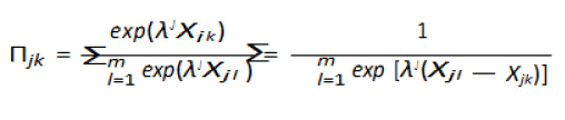
variable. Considering m nominal choices of the response
variable, jk denote the probability that the individual j falls in
category k. Also, let Xj represent the characteristic of individual j.
The probability of the individual
j falling in category k is given by

Here, γ1 γm are m vectors of unknown parameters where each
of the estimates are different even though Xj is constant accross
other categories or choices. The model to be fit.
Modeling our hemophilia a data by GLM
Using GLM method, the list significantly effective variables
ordered as per the p-value of wald chi-square from smallest to
largest in the model are shown in the following Table 6.
| Covariates (Attributes) |
DF |
Wald chi-square |
Pr>chiSq |
| Mutation (Type of protein change) |
6 |
42.5087 |
<0.0001 |
| Domain (Location of mutation domain) |
12 |
24.3374 |
0.0183 |
| Race of individuals |
6 |
13.5698 |
0.0348 |
| Inhibitor history |
2 |
3.2079 |
0.2011 |
| Mechanism (Type of DNA change) |
6 |
5.0811 |
0.5335 |
| Exon (Exon number in the mutation location) |
2 |
1.1978 |
0.5494 |
| Codon (Codon number in the mutation location) |
2 |
0.913 |
0.6335 |
Table 6: Ranking of covariates in the generalized logistic
regression.
Taking statistically significant covariates as per the above into
consideration and letting severe as the reference category of
response variable, the final generalized models are:
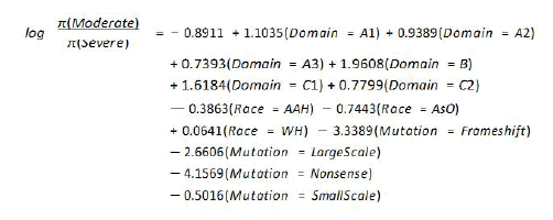
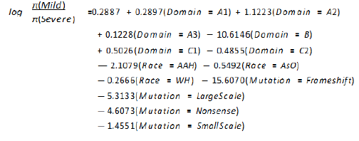
The equation for mild category of response variable where
severe as the base reference category:
Generalized Estimating Equations (GEE)
This modeling technique is widely used in analyzing
longitudinal data when the average effect of population is the
primary interest of the study objectives. Let, yij, j=1 ni and i=1k
represents jth response of the ith subject and has the vector of
attributes xij, then, there are ni measurements on subject i and
maximum number of measurements per subject is T. Also, if μij
is the marginal mean of response yij which is related to a linear
predictor through a link function g(μij)=xJijθ, then the variance of
yij depends on the mean through a variance function v(μij). An
estimate of the parameter θ can be solved by generalized
estimating equations.
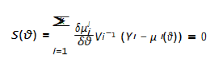
Here, Vi is the covariance matrix of Yi.
Cumulative Logistic Model (CLM)
Suppose, Y takes values of y1, y2,…ym such that y1<y2,<,<ym, it
is assumed that the observed variable is categorized through a
continuous latent variable U such that, Y=yi ⇔ αi-1<U ≤ αi, i=1,
m where −∞=α0<α1<αm=∞. The assumption on U is that the
value will be determined by the attributable variable vector X in
the form of a linear function U=−λjx+ϵ where, λ is vector of
regression coefficients and ϵ is a random variable with a
distribution function F that assumed to follow P(Y ≤ yi|x)=F(αi+jx)
logistic distribution. Moreover, in the CLM concept, alternatively
known as proportion odds model, it is assumed that the
predictor variable, let X, takes different values for each of the
alternative categories and effect of a unit of X is assumed
constant across different alternative categories. Under these
assumptions, the probability that an individual j will fall into
category k is:
Modeling our hemophilia a data by CLM
In order to appy CLM method to our data set at hand, let our
response variable be F8 Severity Level=Yj={yj1, yj2, yj3} where the
ordering is in reverse order of category 1 indicates the most
severe case (Severe) and category 3 indicates least severe (mild).
The associated probabilities are {πj1, πj2, πj3}, and a cumulative
probability of a response less than equal to Yj is:
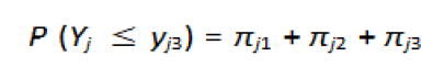
Then the CLM would be:
The sequence of cumulative logit models will be:
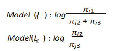
Or alternatively the simplified versions of the above models
can be expressed as by the following equations as well:
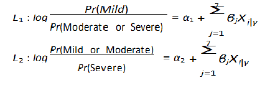
Here, γ is indicator for categories of each categorical variable
and other notations:
Here, we should notice that the intercepts are changing from
one model to another but the slopes are equal for all the
models. Also, we need to estimate 2-intercepts and p-slopes. In
our case p=7, so we will have 7 slopes for 7 covariates and 2
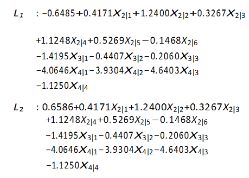
intercepts should make the full model. The estimated final
model is given in equation.
The model given in equation, is formulated considering all the
attributable variables in the given data set of hemophilia A
disease. But if the covariates are ranked based on their effects
on the model, then there are some v ariables which are not
statistically significant. The following represents the ranking of
statistically significant covariates ranked f rom that of the most statistically significant to statisti cally insignificant variables of
(Table 7).
| Covariates (Attributes) |
DF |
Wald chi-square |
Pr>chiSq |
| Mutation (Type of protein change) |
3 |
44.4268 |
<0.0001 |
| Race of Individuals |
3 |
13.5435 |
0.0036 |
| Domain (Location of mutation domain) |
6 |
16.7199 |
0.0104 |
| Mechanism (Type of DNA change) |
3 |
7.1198 |
0.0682 |
| Inhibitor history |
1 |
1.9719 |
0.1602 |
| Exon |
1 |
0.4538 |
0.5005 |
| Codon |
1 |
0.1836 |
0.6683 |
Table 7: Ranking of covariates in the cumulative logistic
regression.
Validation of the proposed model
From the previous section, it is recommended that, in the
modeling purpose with the data set at hand, we should include only 3 IVs (Independent Variables) as per Table , where as that
thestatistically significant variables are ranked as per
their corresponding p-values.
So, by taking this with the significance into considerations the
final proposed model for the hemophilia dataset we have at our
hand is given in the Equation below:
As a part of validation of the model presented in equation,
from it clearly shows the insignificance of the proportional odds
assumption of the cumulative logistics Model and from this fact
it can be concluded that the relationship between Severe
category and mild category or the severe and moderate category
are the same with respect to the proportional odds. In other
words, the co-efficients that describe the relationship between Severe level of disease vs. mild and moderate categories of the response variable (severity level) are the same as those
coefficients that describe the relationship between Moderate
and mild category of response variable which is in other words
called parallel regression assumption as shown in the Figure 8.
Figure 8: Proportional odds assumption for cumulative
logistic regression of hemophilia A. Note: 95% Confidence
limits 95%
prediction limits regression
From the above, it indicates that the proportional odds
assumption is not violated and the diagonal parallel lines
indicate the parallel regression assumptions as well. This is also
confirmed by the chi-square test of the model given in the Table 8.
| Chi-square |
DF |
Pr>chiSq |
| 17.2278 |
13 |
0.1891 |
Table 8: Testing for proportional odds assumption.
Concerning the model fit, AIC, SC, and LogL given in Table 9 indicate that the fitted model is statistically significant also From the model given in equation, it indicates that 1
unit change of domain protein (A2), we expect that there will
be approximately 42% increase in the log odds being in the
lower level of the severity level from sever to mild when all
other covariates are held constant. So, there are always a
positive increase in the log odds for one unit increase in
each of the domain protein category. On the other hand,
one unit increase or change from one category of race to other
category of race will have negative effect in the log odds of
being from mild to moderate category of severity level so is the
third categorical variable, mutation.
| Criterion |
Intercept only |
Intercept and covariates |
| AIC |
1678.152 |
1102.99 |
| SC |
1687.915 |
1176.211 |
| -2 Log L |
1674.152 |
1072.99 |
Table 9: Model fit statistics for hemophilia A data.
Now, we want to rank the attributable variables with respect
to the effects in the model. Table th at shows the ranking of
attributable variables with respect to their p-value in the model.
The first variable in case of GLM is Mutation and last variable is
Codon and it is also the same when the modeling is done with
CLM also. But things to be noted in CLM method is that the
ranking of statistically significant variables changes as the
modeling technique changes. For example, the third variable in
GLM from top is Race of individuals, but in CLM method, the
third variable from top is Domain (Location of Mutation Domain)
at 5% level of significance.
Here, for instance, it is very important to discuss the proposed
model given in equation and model in equation the following
table shows the comparison of some vital information about the
full model and the model that is built considering the
statistically significant covariates only (Table 10).
| Model |
|
CLM (All covariates) |
CLM (Only sig. covariates) |
| % Concordant |
81.4 |
85.8 |
| % Discordant |
17.8 |
10.3 |
| % Tied |
0.8 |
3.9 |
| Somers’ D |
0.63 |
0.75 |
| C(ROC) |
0.81 |
0.87 |
Table 10: Comparison of association of predicted probabilities and observed responses.
Discussion
From the table above, we can see that the percentage of
concordant pairs of CLM while considering all the covariates in
the model is approximately 4% less than that of the CLM built
with statistically significant covariates. Also, % of area covered
under the ROC curve is 6% higher in CLM with significant
variables than that of the CLM with all covariates. After
comparing the statistic given in it is statistically conclusive that
the model given in equation is a better predictive model to
predict the probability of the severity level of hemophilia A with
F8 as per our dataset at hand.In terms of finding the best model
driven by our data at hand, the Cumulative Logistic Regression
considering the statistically significant covariates only as the
independent variables has fast convergence rate and best
results based on our data apprently. This model is predicting
the probability for each of the response category with about
87% accuracy under the ROC as per C statistic.
In the context of the disease, the model given in Equation, has
not violated the proportional odds assumption of the CLM. In
brief, as per model given in the equ ation it indicates
that, protiens A1, A2, A3, B, C1 of Domain mutation will
effect the probability of severity level of any individual in an
increasing manner, i. e., if the doctors and scientists can
identify these protiens in the blood then they have to
provide some treatments that will locate these protiens
and reduce their positive effects to increase patients
probability of being in the mild category (lowest category of
severity level in hemophilia A) from very severe category of
the disease and it has to be opposite in case of C2
protien to improve or alleviate the severity level of any
patient. As per model in Equat ion race is affecting the
probability of individuals being in one of the three categories
of response variable and there are no real life treatment of to
chang race of individuals we might counclude that being in
the different categories of Severity level by race categories
are totally in hands of mother nature. But, it is conclusive
that majority of patients in sever cateogry comes from white
non-hispanic rather than other categories of race. On the other
hand, the (Nonsense) has the smallest coefficient in the
model mentioned above indicates that Nonsense type
mutation change in the gene of individual will have maximum
effect on the response outcome and to change/alleviate the
severity level of any individual, it is suggested to attack/reverse
this particular type of mutation cause and consequently change
other types of mutaions.
Conclusion
The objectives of this study were to indentify statistically signifi--cant variables that effects the outcome variable “Severity
Level”. Also, we wanted to see statistically significant
categories of variables interacting with each other effecting
the categories of response variable if any. At the same time we
wanted to rank the main effect variables that are contributing
to the response and eventually come upe with a model
that is statistically siginificant and robust with high degree of
prediction porbability prediction and convergence. So, we have
indentified statistically significant variables that effects
the Severity Level by implementing various methodology
for model building and we have compared them through
some statistic. It turns out that the attributable variables
Race, Domain and Mutation type are the most significant
variables to predict the probability of the severity level of
hemophilia A statistically shown in Tables. Also, we have
investigated the interaction terms among the
attributable variables and it turns out that there were no
interactions among variates as per out data concerns.
In terms of practical relevancies, our model will predict the
probability of severity level of any individuals with 87% accuracy.
So, if any individual goes to Medical doctor and after getting the
results of blood diagnosis and if the individual provides available
information on Domain (Location of mutation change), Mutation
(Type of Protein change) and Race of individuals then Medical
doctors will be able to identify the Level of Severity for
that particular individual and based on this medical physician
will be able decide proper treatment program for that
individual afetr having the genetic profile analyzed.
REFERENCES
- Robert D Abbott (1985) Logistic regression in survival analysis. Amer J Epidemiol 121: 465-471.
[Crossref][Google scholar][Pubmed]
- Cande V Ananth, David G Kleinbaum (1997) Regression models for ordinal responses: A review of methods and applications. Int J Epidemiol 26: 1323-1333.
[Cross ref][Google cholar][Pubmed]
- Ralf B, Ulrich G (1997) Ordinal logistic regression in medical research. J Royal College Phys London 31: 546–551.
[Google scholar][Pubmed]
- Dankmar Boohning (1992) Multinomial logistic regression algorithm. Annals inst Stat Math 44: 197-200.
[Crossref][Google scholar][Indexing at]
- Norman E Breslow, Nicholas E Day (1980) Statistical methods in cancer research. Vol. 1. The analysis of case-control studies., volume 1. Distributed for IARC by WHO, Geneva, Switzerland. [Cross ref]
[Google scholar][Pubmed][Indexing at]
- A Coppola, M Margaglione, E Santagostino, A Rocino, E Grandone (2009) Factor viii gene (f8) mutations as predictors of outcome in immune tolerance induction of hemophilia a patients with high-responding inhibitors. J Thrombo Haemostat 7: 1809–1815.
[Cross ref][Google scholar][Pubmed]
- Michael Friendly (1994) Mosaic displays for multi-way contingency tables. J Amer Stat Asso 89: 190-200.
[Crossref][Google Scholar][Indexing at]
- AC Goodeve, PH Reitsma, JH McVey (2011) Nomenclature of genetic variants in hemostasis. J Thrombo Haemostat 9: 852-855.
[Cross ref][Google scholar][Pubmed]
- Samantha CG, HM VandenBerg, J Oldenburg, J Astermark, PG deGroot, et al. (2012) F8 gene mutation type and inhibitor development in patients with severe hemophilia a: Systematic review and meta-analysis. Blood 119: 2922-2934.
[Crossref][Google Scholar][Pubmed]
- James W Hardin, Joseph M Hilbe (2002) Generalized estimating equations. Chapman Hall/CRC.
[Crossref][Google scholar][Indexing at]
- ND Hicks, WR Pitney (1957) A rapid screening test for disorders of thromboplastin generation. Br J Haematol 3: 227-237.
[Crossref][Google Scholar][Pubmed]
- Kung-Yee Liang, Scott L Zeger (1986) Longitudinal data analysis using generalized linear models. Biometrika 73: 13-22.
[Crossref][Google scholar][Indexing at]
- Daniel L McFadden (1984) Econometric analysis of qualitative response models. Handbook Econometrics 2: 1395-1457.
[Crossref][Google scholar][Indexing at]
- Richard D McKelvey, William Zavoina (1975) A statistical model for the analysis of ordinal level dependent variables. J Math Socio 4: 103-120.
[Crossref][Google scholar][Indexing at]
- Ann A O’Connell (2006) Logistic regression models for ordinal response variables. Number 146. Sage.
[Google scholar[Indexing at]
- AB Payne, CH Miller, FM Kelly, J M Soucie, WC Hooper, et al. (2013) The cdc hemophilia a mutation project (champ) mutation list: a new online resource. Human Mutation 34: E2382-E2392.
[Crossref][Google scholar][Pubmed]
- John Schwarz, Jan Astermark, Erika D Menius, Mary Carrington, Sharyne M Donfield, et al. (2013) F8 haplotype and inhibitor risk: results from the hemophilia inhibitor genetics study (higs) combined cohort. Haemophilia 19: 113-118.
[Crossref][Google scholar][Pubmed][Indexing at]
- Ying So, Warren F Kuhfeld (1995) Multinomial logit models. In SUGI 20 Conference Proceedings 1227-1234.
[Google scholar][Indexing at]
- Ther`ese A Stukel (1988) Generalized logistic models. J Amer Statist Associat 83: 426-431.
[Crossref][Google scholar][Indexing at]
- Joffre Swai, Jordan Louviere (1993) The role of the scale parameter in the estimation and comparison of multinomial logit models. J Market Res 30: 305-314.
[Cross ref][Google scholar][Indexing at]
- Scott L Zeger, Kung-Yee Liang (1986) Longitudinal data analysis for discrete and continuous outcomes. Biometrics 121-130.
[Cross ref][Google scholar][Pubmed]
- Scott L Zeger, Kung-Yee Liang, Paul S Albert (1988) Models for longitudinal data: A generalized estimating equation approach. Biometrics 1049-1060.
[Crossref][Google scholar][Pubmed]
Citation: Bashar AKMR, Tsokos CP (2022) Statistical Model for Detecting Probability of Severity Level of Hemophilia A. Health Sci J. Vol: 16 No: 7:
963.