Journal of FisheriesSciences.com

Keywords

Fisheries; Commercial catch; By-catch; Length-weight relationship; Linear regression; length/weight sample data; Fish condition; Stock assessment; Biological objects; Statistical analysis; MATLAB; Algorithm

Introduction

Fisheries science states that as fish grow in length they increase in weight and also affirms the functional relationship between length and weight of fish is not linear and can be expressed as:

W(i) = q * L(i)b (1.0)

Where: W(i) is the body weight of a fish, L(i) is the total length and q and b are parameters. The exponent b is stated to be close to 3.0 for most species, however coefficient q varies between species. If the exponent b (or allometric coefficient) is greater than three for a certain fish species, that species tends to become relatively fatter or have more girth as it grows longer (Anderson and Neumann, 1996; Sparre and Venema, 1998).

Since the Length-Weight functional relationship (1.0) is nonlinear the coefficients q and b cannot be obtained directly, and therefore, it needs to be further transformed into a linear equation by taking logarithms of both sides:

lnW(i) = lnq + b*lnL(i)     (1.1)

which gives linear regression model of the following type:

y(i) = a + b*x(i)      (1.2)

Where: y(i) = lnW(i) , x(i) = lnL(i) and a = lnq .

The mathematical transformation (1.1) makes it possible for a and b to be estimated through the use of linear regression analysis, based on sample data (length-weight measurements of fish).

The research on length-weight relationship of fish dates back to the late 1900s, and it was recognized as a decisive tool for describing key biological aspects: estimating the fish weight based on the basis of the length measurements and vice versa, conducting growth pattern analysis using the allometric coefficient of the analyzed species, obtaining an assessment of the body conditions of the sampled fish specimens (i.e. fat storage or gonadal development etc.). Furthermore, the knowledge acquired as a result of the study into the length-weight relationship is essential for the provision of fish stocks assessments, for developing fish stocks condition analysis and performing strict fisheries monitoring programs (Froese, 2006).

Fish condition is an extremely important fish population parameter, for which fisheries scientists are expected to make further management recommendations. Few condition indices have been found useful for measuring fish condition – Fulton condition factor: 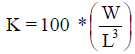, it assumes isometric body growth (i.e. b = 3) , or that fish body does not change with the body growth and is calculated as ratio between the observed weight and the expected weight in relation to the body length. There are other indices introduced as well: Relative condition factor Kn = W/W', where W is the observed weight of individual fish and W' is the predicted, length-specific mean weigh for the population under study; and the relative weight 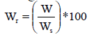, where: W is the observed weight and s W the reference standard weight value for fish of the same weight (Blackwell, Brown, Willis, 2000). For the provision of accurate body condition analysis based on weight estimates it is important that the length-weight conversion models are properly investigated and statistically validated.

The present article deals with Length-weight relationship analysis of commercial fisheries samples (length/weight frequency samples) of species taken from commercial catch caught in the Bulgarian part of the Black sea–i.e. sprat as a targeted catch and anchovy as by-catch. The samples are analyzed by the available engineering approaches in statistical modeling, system identification and system modeling (Genov, 2000). The term biological object (BO) refers to the species under examination and is introduced with a view to simplicity and brevity of the presentation. Sprat and anchovy are considered as being among the most abundant species in the Black sea with the sprat being also subject of maximum sustainable yield (MSY) limitations. Sprat stock has been assessed on semi-annual basis since 2007 in order to facilitate proper MSY recommendation.

Short biological characteristics of sprat (BO1)

Sprat is an abundant and widely distributed fish along the European coastlines of the Mediterranean, especially the Adriatic and the Black Sea. Sprat is a small pelagic marine fish with a body length, as most presented in commercial fisheries and trawl surveys, varying between 8 and 10 cm (depending on the gear selectivity) and it weights around 9-10 grams. Its lifespan lasts approximately for 4-5 years (Raykov and Yankova, 2006).

Short biological characteristics of anchovy (BO2)

Anchovy is a small pelagic fish in all shelf areas surrounding Europe from the North African upwelling and the Black Sea north to the Baltic Sea and southern Norwegian coasts. The anchovies are known to be shifting their distributions to the north. They are regularly caught on the Coasts of Bulgaria, Croatia, Georgia, Romania, Russia and Turkey. Black sea adult anchovies can reach a body length of 12-15 cm. The stock is differentiated into 4 age groups in most survey data – the highest age class is identified 4+ (Froese and Pauly, 2017).

Methods

An experimental approach was adopted for collecting data (body length and body weight measurements of BO1 and BO2) to support the length-weight relationship analysis for statistical purposes. The samples are taken from commercial catches (stationary pound nets -7, 5 mm mesh size). The fish was caught on 1st of May 2017, near Varna, Bulgaria - “Trakata” area. The catch composition involved two species (BO)-Sprat (BO1) as a targeted catch and anchovy (BO2) as a by-catch. The samples processed for further analysis are: n=1000 individuals of BO1 and n=230 individuals of BO2.

The overall aim of the first stage of the research was to investigate the type of the functional relationship (i.e. to derive a mathematical model) by direct application of a linear regression analysis; and that of the second stage was to validate the model presented with eq. (1.0) for BO1 and BO2, based on the sample data gathered during the experiment.

The analysis is supported by relevant software development in MATLAB environment using regression in matrix form and statistical validation and interpretation of the results delivered. The developed algorithm works well with natural, standardized and log-transformed values of the variables under investigation. The process of ascertaining and the relevant statistical analysis of the mathematical models were carried out in two stages:

Stage 1: Applying initial analysis of the mathematical relationship between length and weight (assuming linear relationship, which is to be further proven) by using linear regression, based on the experimental data, and statistical analysis of the overall significance of the model employed for the purpose of the research;

Stage 2: Investigation of validity of eq. (1.0) by linear regression analysis of the log-transformed length-weight experimental data, further determination of the regression coefficients and provision of the statistical analysis as to the overall significance of the given model;

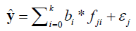
The normal error linear regression model can be expressed as:

     (1.3)

and can be derived from the following calculation procedure by the use of the matrix approach.

Determine regression coefficients

Form the input-output data vectors:

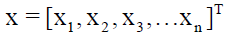- input vector of the independent variable x (x = L - length measurements)

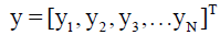- output vector of the dependent variable y (y = W - weight measurements) .

- Create the experiment matrix X and the regression matrix F:

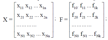
Determine the coefficients bi of the model     (1.3)

b = C*FT * y      (1. 4)

Where: C = (FT *F)-1 is the covariance matrix, the determinant of (FT *F) must be ≠ 0 and its condition number <10-102 (Belsley et al., 1980).

Analysis of the overall statistical significance of the mathematical model delivered

Calculate the total sum of squares Q:

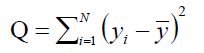(1.5)  

Where is the mean value of the output variable and is obtained with:

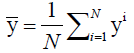
- Calculate the partition of the sum of squares:

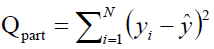(1.6)

Where: are the values of the output variable assessed by the model delivered.

calculate the correlation coefficient R , which is a measure for determination of the mathematical model obtained;

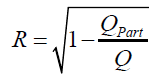(1.7)

F-test of the overall model significance:

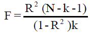    (1.8)

The critical value is found in F-distribution table for significance level α = 0.05 and degrees of freedom and.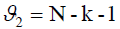

If F > Fc , the calculated value of R is assumed significant for α = 0.05 , and proves that the model delivered by using the above described calculation procedure is adequate (Genov, 2000).

Program Development Using Matlab

The following step algorithm is used for specific software development in MATLAB programming environment to execute the calculation procedure and the statistical analysis that were mentioned earlier in the paper.

Investigation of linear length-weight relationship model validity using linear regression analysis of L(x) as independent variable and W(y) – as a dependent variable (direct measurements)

Step 1: Process the length-weight measurements of sample data for BO1 and BO2 to form input/output vectors to be used as a basis for regression analysis – saved in separate .mat-files named ‘SpratLW.mat’/’AnchovyLW.mat’.

Step 2: Form the regression matrix and check if the system of equations is well-conditioned.

Step 3: Determine the regression coefficients.

Step 4: Calculate the correlation coefficient as a measure of determination of the model obtained.

Step 5: F-statistics (F-test the overall model significance).

Step 6: Calculate 95% confidence limits for the regression coefficients.

Investigation of non-linear length-weight relationship model validity eq. (1.0) by linear transformation of (1.0) an linear regression of log transformed length-weight data, analyzing L(x) as independent variable and W(y) – as a dependent variable

Step 1: Log-transformation of the Length-weight data collected for BO1 and BO2.

Step 2: Form the regression matrix.

Step 3: Determine the regression coefficients.

Step 4: Calculate the correlation coefficient as a measure of determination of the model obtained.

Step 5: F-statistics (F-test the overall model significance).

Step 6: Calculate 95% confidence limits for regression coefficient b.

Step 7: Calculate linear and non-linear model errors.

The MATLAB Program Script Written for the Purpose of this Analysis is Presented Below

function LenghtWeightLIN_NONLIN1(tn2,n,W,L)

%LENGTH/WEIGHT RELATIONSHIP (LWR) ANALYSIS OF COMMERCIAL FISHERY SAMPLES

%TAKEN FROM THE BLACK SEA (BULGARIA)- Sprat and Anchovy case study%

%1. Investigation on linear LWR model validity - regression analysis of L(x) against W(y) (observations)*%

clc

clear

load('spratLW.mat')

Lmean=mean(L);%Calculates the Mean value of L%

Wmean=mean(W);%Calculates the Mean value of W%

sL=std(L);%Calculates the standard deviation of x=L%

%Regression analysis%

f0=ones(n,1);

F=[f0,L]; %Forms the Regression Matrix%

FFl=F'*F;

b=(((FFl)^(-1))*F')*W %Claculates regression coefficients%

beta=b';

b0=beta(1,1)%displays regression coefficient b0 value%

b1=beta(1,2)%%displays regression coefficient b1 value%

Cond=cond(FFl)%determines the condition factor of the information matrix FFl, which forms the covariance matrix, once inverted - if the condition factor cond(FF) >10-10^2 it is reccomended to run the analysis with normalized/standardized %

%x (L) values of the independent variable to overcome the problem with numerical calculations and analysis%

%Cond FFl= 2.1218e+004 > 10 to 10^2 ==> normalized X values will be used to %validate the regression coefficients estimates%

%Regression analysis using the normalized X=L values %

f0=ones(n,1);

Lnorm=(L-Lmean)/sL;%normalizes the independent variable L values%

Fnorm=[f0,Lnorm];%forms the regression matrix by using the normalized values of the independent variable%

FFnorm=Fnorm'*Fnorm;

Cond_norm=cond(FFnorm)%Cond(FFnorrm)=1.0044 < 10- 10^2 → the matrix is well conditioned%

B=(((FFnorm)^(-1))*Fnorm')*W %calculates the regression coefficients%

Bl=B'

b0l=Bl(1,1)%displays regression coefficient b0 value%

b1l=Bl(1,2)%displays regression coefficient b1 value%

B0l=(b0l-((b1l*Lmean)/sL))%validates b0 value%

B1l=b1l/sL%validates b1 values%

Whatl=B0l+(B1l*L);%Calculates What=Westimated by the model values with the validated coefficients b0 and b1 (y=b0+b1*x)%

el=W-Whatl;%Calculates the error between the measured and estimated

%by the model values%

%Statistical analysis of the overall model significance%

Qpartl=sum((W-Whatl).^2); %Calculates the partition of the sums of squares%

Ql=sum((W-Wmean).^2);%Calculates the total sum of squares%

Qcalcl=Qpartl/Ql;

Rl=sqrt((1-Qcalcl))%Calculates the correlation coeficient%

%F-tests the overall model signifficance%

Fl=(Rl^2*(n-2))/((1-Rl^2)*1)%Fc is found in F-test distribution table to be compared%

%with the calculated value Fl%

%grahic representation of W (measured) and What (estimated) by the model values vs. L (measured)%

figure

scatter(L,W);grid

title('Linear Model fit over the actual data:W_m_e_a_s_u_r_e_d,L and W_e_s_t_i_m_a_t_e_d by the model, L') hold on

y1 = Whatl;

plot(L,y1)

hold off

%Constructs the Regression coefficients (b0 and b1) 95% confidence intervals %

%Calculates the variance and standard deviations of L,W,b0 and b1%

sL=std(L);%standard deviation of L%

sL2=sL^2;%variance of L%

sW=std(W);%standard deviation of W%

sW2=sW^2;%Variance of W%

sb12=(sW/sL).^2)-(b1.^2))/(n-2);%variance of b1%

sb1=sqrt(sb12);%standard deviation of b1%

%student distribution 95% tn-2 (table value=1.960)%

%calculates the confidence interval for b1%

Sb1tn2=sb1*tn2;

CIlowb1=b1-Sb1tn2

CIupb1=b1+Sb1tn2

%calculates the confidence interval for b0%

sb02=sb12*((((n-1)/n)*sL2)+Lmean);

sb0=sqrt(sb02);%variance of b0%

Sb0tn2=sb0*tn2;%standard deviation of b0%

CIlowb0l=b0-Sb0tn2

CIupb0l=b0+Sb0tn2

%2. Investigation on nonlinear LWR model W=q*L^b validity**%

Wi=log(W(:,1));%takes logarithm on W-measurements%

Li=log(L(:,1));%takes logarithm on L-measurements%

Lmeann=mean(Li);%calculates the Mean value of Li%

Wmeann=mean(Wi);%Calculates the Mean value of Wi%

%Regression analysis%

x0=ones(n,1);

X=[x0,Li];%Forms the regression matrix%

XXn=X'*X

b=((XXn)^(-1))*X'*Wi; %Claculates regression coefficients%

beta=b';

b0n=beta(1,1);

b1n=beta(1,2);

a=b0n;

br=b1n%displays coefficient b%

q=exp(a)%calculates the coefficient q%

Whatn=a+(br*Li);%What=Westimation - estimates W by the model derived%

e=Wi-Whatn;%calculates the model error%

%Statistical analysis of the overall model significance%

Qpn=sum((Wi-Whatn).^2); %Calculates the partition of the sums of squares%

Qn=sum((Wi-Wmeann).^2);%Calculates the total sum of squares%

Qcalcn=Qpn/Qn;

Rn=sqrt((1-Qcalcn))%Calculates the correlation coefficient%

%F-tests the overall model signifficance%

Fn=(Rn^2*(n-2))/((1-Rn^2)*1)%Fc is found in F-test distribution table to be compared%

%with the calculated value Fn%

%Calculates 95% Confidence interval for allometric coefficient b%

sL=std(Li)%calculates the standard deviation of L%

sL2=sL^2;%calculates L variance%

sW=std(Wi)%calculates the standard deviation of W%

sW2=sW^2;%calculates W variance%

sLW=sW/sL;

s2=sLW.^2;

br2=br.^2;

sb2=(s2-br2)/(n-2); %calculates the variance of b%

sb=sqrt(sb2);%calculates the standard deviation of b%

%student distribution 95% tn-2 (table value=1.960)%

%calculates the confidence interval for the coefficient b%

CI95=sb*tn2;

CI95downn=br-CI95

CI95upn=br+CI95

%Calculation of Weight by using the values of q and b, obtained by the regression analysis and the measured values of L %

Wn=q*L.^br;

%Graphic representation of the model fit Wn over the actual data (observations of W and L)%

figure

scatter(L,W);grid

title('Non-linear Model fit over the actual data:W_m_e_a_s_u_r_e_d,L and W_e_s_t_i_m_a_t_e_d by the model,L')

hold on

y1 = Wn;

plot(L,y1)

hold off

en=W-Wn;%calculates the model error%

x=1:n;

%graphic representation of the model error (linear and nonlinear LWR)

figure

plot(x,el);grid

title('Linear model error e_l and nonlinear model error e_n')

hold on

y1 = en;

plot(x,y1)

hold off

end

*Index “l” stands to indicate estimates and parameters introduced in the Linear Length-weight relationship model analysis.

**index “n” indicates estimates and parameters introduced in the non-linear Length-weight relationship model.

Results

Length-weight relationship analysis of BO1

Regression analysis and F-statistics results delivered for both linear and non-linear models are presented in Table 1.

Linear model analysis results for BO1 (n=1000)	Non-linear model analysis results for BO1 (n=1000)
Intercept b = -10.6120	Coefficient   q = 0.0042
Regression coefficient b = 1.7092	Coefficient b = 3.1876
Linear regression model: WLin= -10.6120+1.7092 * L	Non-linear model: WNon = 0.0042 * L3.1876
Correlation coefficient: R=0.8648	Correlation coefficient: R=0.8662
F-statistics calculated value:Fl = 2.9596e + 003	F-statistics calculated value: Fn = 2.9998e + 003
F-statistics critical value:Fc = 3.85	F-statistics critical value: Fc = 3.85
95% Confidence interval b0=[-10.8043;-10.4196]	95% Confidence interval b=[ 3.0736;3.3017]
95% Confidence interval b1=[ 1.6476;1.7708]	Conclusion: the Non-linear model delivered: WNon= 0.0042 * L3.1876is statistically significant and adequate and is proved valid with sufficient precision for BO1(sprat).
Conclusion: the linear model delivered: WLin= -10.6120 + 1.70 * L is statistically significant and adequate enough to describe the Length-weight functional relationship of BO1(sprat) with sufficient preciseness.

Table 1: Length-Weight relationship analysis results for BO1.

Graphic presentation of linear and non-linear model fit over the actual (observed) data is shown in Figure 1 for linear model and in Figure 2 for the non-linear model investigated. The errors calculated for both – linear and nonlinear Length-weight relationship models delivered by the analysis of BO1 sample data are shown in Figure 3.

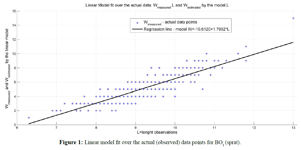
Figure 1: Linear model fit over the actual (observed) data points for BO1 (sprat).

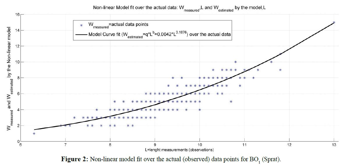
Figure 2: Non-linear model fit over the actual (observed) data points for BO1 (Sprat).

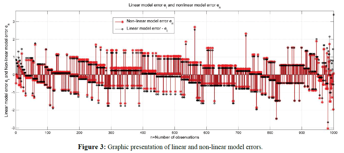
Figure 3: Graphic presentation of linear and non-linear model errors.

Length-weight relationship analysis of BO2

Regression analysis and F-statistics results delivered for both linear and non-linear models are presented in Table 2. Graphic presentation of linear and non-linear model fit over the actual (observed) data is shown in Figure 4 for linear model and in Figure 5 for the non-linear model investigated. The errors calculated for both-linear and nonlinear Length-weight relationship models delivered by the analysis of BO2 sample data are shown in Figure 6.

Linear model analysis results for BO2 (n=230)	Non-linear model analysis results for BO2 (n=230)
Intercept b0=-17.6912	Coefficient  q=0.0072
Regression coefficient b1=2.2893	Coefficient b = 2.8906
Linear regression model: WLin=-17.6912+2.2893*L	Non-linear model: WNon= 0.0072 * L2.8906
Correlation coefficient: R=0.9204	Correlation coefficient: R=0.9284
F-statistics calculated value: Fl = 1.2636e + 003	F-statistics calculated value: Fn = 1.4244e + 003
F-statistics critical value: Fc = 3.92	F-statistics critical value: Fc = 3.92
95% Confidence interval b0 = [-18.1485;-17.2339]	95% Confidence interval b = [ 2.7405;3.0408]
95% Confidence interval b1 = [2.1630; 2.4155]	Conclusion: the Non-linear model: WNon = 0.0072 * L2.8906 is statistically significant and adequate and is proved valid with sufficient precision for BO2 (anchovy).
Conclusion: the linear model: WLin = -17.6912 + 2.2893 * L is statistically significant and adequate enough to describe the Length-weight functional relationship of BO2 (anchovy) with sufficient preciseness.

Table 2: Length-Weight relationship analysis results for BO2.

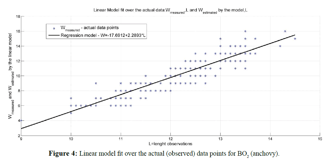
Figure 4: Linear model fit over the actual (observed) data points for BO2 (anchovy).

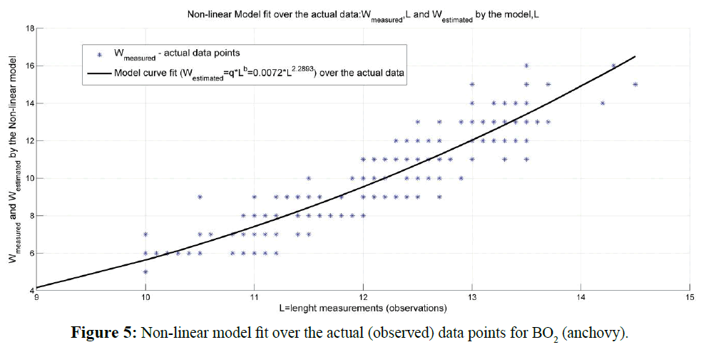
Figure 5: Non-linear model fit over the actual (observed) data points for BO2 (anchovy).

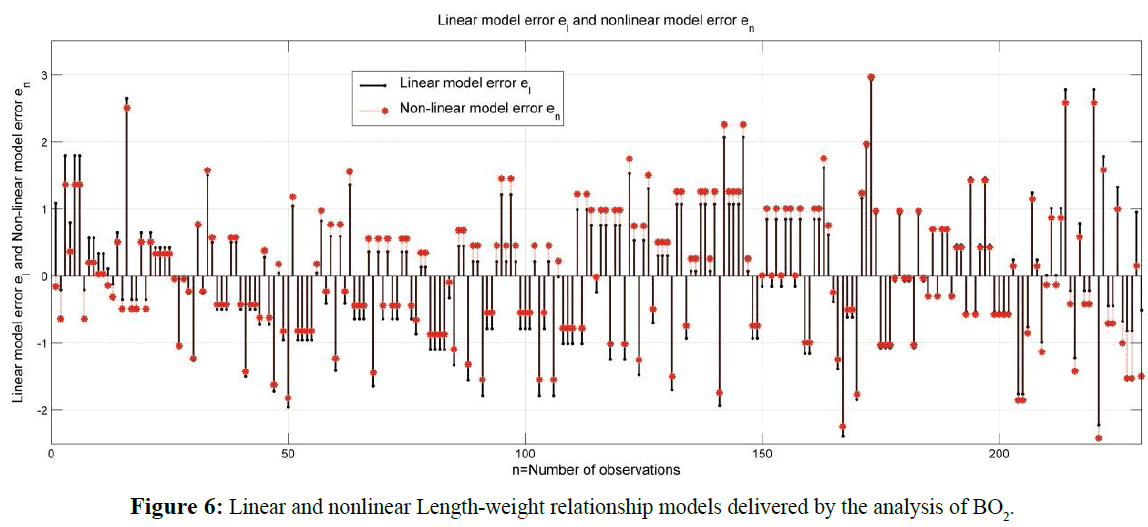
Figure 6: Linear and nonlinear Length-weight relationship models delivered by the analysis of BO2.

Discussion

In the linear regression analysis (stage 1 of the present research), the matrix (FT *F) is found to be with a large condition number or ill-conditioned for both BO: Cond(FT *F)BO1 =1.4779e + 0;04Cond(FT * F)BO2 = 2.1218e + 004 . It is known that in the field of numerical analysis, the condition number of a function with respect to an argument measures how much the output value of a certain function can change for a small change in the input argument. This is used to measure how sensitive a function is to changes or errors in the input, and how much error in the output results from an error in the input. In linear regression the condition number can be used also as a diagnostic for multicollinearity. If the condition number of a matrix is not too much larger than one, the matrix is well conditioned which means its inverse can be computed with considerable accuracy. If the condition number is very large, then the matrix is said to be ill-conditioned. Practically, such a matrix is almost singular, and the computation of its inverse or solution of a linear system of equations is prone to large numerical errors. When the condition number is equal to one, then a solution algorithm can find (if it does not introduce errors of its own) an approximate solution whose precision corresponds to the accuracy of the data analyzed (Belsley et al., 1980; Pesaran, 2015). To overcome the problem implemented are standardized variables within the algorithm under examination. Standardizing or normalizing of variable in mathematic terms implies the analysis of a scaled (normalized) variable, calculated by subtracting mean of the original variable from the raw (measured/observed) value and its subsequent division it by original variable standard deviation:

where: is the raw (measured) value of the input variable, is the mean and is the standard deviation (Genov, 2000). The analysis with implemented normalized variables prove to facilitate Cond(FT *F)norm = 1.0044 for both BO, which in turn leads to conclusion that the algorithm delivers an approximation of the solution whose precision is no worse than that of the data or it does not introduces errors of its own.

Conclusions

The first stage of analysis of Length-weight relationship of BO1 and BO2 sample data delivered two statistically significant and adequate linear models, which might be successfully used for conversion of the Length into Weight and vice versa, valid for analyzed species, should we consider this validity only within their exploitation phase.

The second stage of analysis as regards the non-linear relationship model validity (eq. 1.0) proves that the non-linear model W(i) = q*L(i)b is also valid for the reviewed BOs and the linear regression model used for calculation of the coefficients q and b is statistically significant and entirely adequate.

A comparison between the weight estimates derived by the two models shows

The linear model can be successfully implemented for conversion of length to weight and vice versa on condition that such a model is applied only for the lengths and weights specific for the exploitation phase of the BO under analysis (for lengths above 7.5 cm for sprat and lengths above 10 cm for anchovy) and tends to deliver non-realistic values for pre-recruitment stage specific lengths.

Non-linear model delivers slightly overestimated values of weight for higher length classes of BO2 for lengths above 14.5 cm.

Both models produce weight estimates with acceptable accuracy for lengths specific for the exploitation phase-the linear one delivers exact or slightly lower values as compared to those under observation, and the non-linear one delivers exact or slightly overestimated values than those of the surveyed individual lengths.

On the whole, since the two models are significant and adequate under certain conditions the appropriate selection of one model over the other with a higher precision of the estimates is, therefore, achievable should the analysis is done on a much more frequent terms or on a yearly-basis taking into consideration the environmental and climatic changes as well as the corresponding growth patterns. It is possible that both linear and non-linear length weight functional relationships are likely to be valid for most small pelagic species and if seasonal growth and favorable environment are taken into account for a certain seasons one might describe the length-weight relationship better than other, but both are still valid on annual basis.

Accordingly, a specific program was developed for execution and automatic rendering of analysis results which might be successfully applied to other cases, once the measurements are processed, saved and loaded in the program as file type ‘.mat’ and the name of the program is simply typed in MATLAB workspace (it will be executed automatically and the results will appear in the workspace). Finally, the program is developed in such a manner to overcome typical calculation problems in numerical analysis and to ensure that no calculation error is added to the solution constructed through the proposed algorithm.

20582

References

1. Anderson, RO., Neumann, RM. (1996) Length, Weight, and Associated Structural Indices, in: B.E. Murphy and Willis DW (editor): Fisheries Techniques, 2nd edition, Am Fisheries Soc Bethesda, Maryland pp: 447-481.
2. Belsley, DA., Kuh, E., Welsch, RE. (1980) The Condition Number. Regression Diagnostics: Identifying Influential Data and Sources of Collinearity. John Wiley & Sons, New York.
3. Blackwell, BG., Brown, ML., Willis, DW. (2000) Relative Weight (Wr) Status and Current Use in Fisheries Assessment and Management, Rev Fisheries Sci 8, 1-44.
4. Cheney, W., Kincaid, D. (2008) Numerical Mathematics and Computing, 6th edition. Thomson Brooks/Cole.
5. Froese, R. (2006) Cube law, condition factor and weight-length relationships: history, meta-analysis and recommendations. J Applied Ichthyol 22, 241-253.
6. Froese R., Pauly D. (2017) FishBase (version Feb 2017). In: Roskov Y., Abucay L., Orrell T., Nicolson D., Bailly N., Kirk P.M., Bourgoin T., DeWalt R.E., Decock W., De Wever A., Nieukerken E. van, Zarucchi J., Penev L., (editors) (2017). Species 2000 & ITIS Catalogue of Life, 26th July 2017. Digital resource at www.catalogueoflife.org/col. Species 2000: Naturalis, Leiden, the Netherlands.
7. Genov, D. (2000) Modeling and Optimization of industrial processes Manual Lab, Varna: Technical university-Varna p: 192.
8. Pesaran, MH. (2015) The Multicollinearity Problem. Time Series and Panel Data Econometrics. New York: Oxford University Press pp: 67-72.
9. Raykov, V., Yankova. M. (2006) Biometric properties of the Sprat, (Sprattus sprattus L.) Off the Bulgarian Black Sea coast. Cercetary marine 36, 349-362.
10. Sparre P., Venema SC. (1998)  Introduction to Tropical Fish Stock Assessment - Part 1: Manual. Rome: FAO Fish Tech Pap p: 407.