Health Science Journal

Keywords

Agent-based simulation; Cancer evolution model; Colon cancer; Colorectal cancer; Virtual patient

Introduction

Almost half Canadians (41% women and 46% men) will develop cancer during their lifetime and 88% of them are older than fifty [1]. Lung, breast, colon, colorectal and prostate cancers represent more than half of all new cancer cases (52%). Breast cancer is the leading type of cancer among women, while colon and colorectal cancer are the third most common cancer among men and women. Cancer is the leading cause of death in Canada and in the world with 29.8% of the population affected, compared to 26.6% for cardiovascular diseases [2]. Furthermore, in 2000, cancer was the fourth most expensive disease in Canada with $17.4 billion spent. Colon and Colorectal cancer are considered the second leading cause of cancer death among men and the third among women.

Cancer treatment is characterized by the convergence of many services including ambulatory, hospitals, clinical, nutritional, psychological, and sports medicine, which coordination and integration condition treatment success and patient quality of life. In order to reduce the impact of this disease and increase the cure rate and the patient quality of life, it is necessary to develop and evaluate new therapeutic and organizational approaches. This study deals with this goal and is the first methodological step toward creating a simulation platform of care trajectories of colorectal cancer patients. This simulation platform aims at simulating many elements of the hospital environment, from care resources to patient physiology and psychology profiles, in order to evaluate the many impacts of organizational changes of care trajectories.

First, this paper describes the general scope of this simulation project and presents a state of the art of agentbased simulation. Next, the general conceptual model of the simulation is described. Then, we present our cancer evolution, which is then tested and validated using two separate experiments.

Research Objective and General Methodology

This section introduces the general objectives and limits of this study and presents the general methodology used to achieve the objectives.

Project general and specific objectives

Providing high-quality care is a priority among health professionals. However, resources are limited and their utilization must be optimized in order to meet high quality standard and patients unique profile. Therefore, the challenge faced by care providers and managers is to design organizational and medical processes that will deliver the right treatment, to the right patient, at the right time using the right resources. This study is part of a comprehensive project, which aims at developing a computer simulation environment of patient care trajectories in order to evaluate new approaches to increase hospital productivity and adapt hospital clinical practice conditions for the elderly and patients with multiple chronic diseases.

Ultimately, the simulation model will include:

1. The physical health of the patient;

2. The cognitive state of the patient;

3. The psychosocial state of the patients;

4. The hospital resources, staff and physicians.

In other words, factors such as socio-demographic and environmental characteristics, as well as the characteristics of the organizational and decision-making systems, will be used to simulate patient care trajectories, from their diagnosis to the end of the treatment. The expected result of this project is an innovative modeling of the interactions between the patients and the health care system, and ultimately, the development and validation of a new approach of providing cares. This simulation environment will support the simultaneous optimization of resources utilization and care quality by assessing the performance of multiple patient care trajectories in a virtual hospital based on reengineered organizational and medical procedure of the Montreal General Jewish Hospital. This paper focuses specifically on the first developmental step of this simulation model, which concerns the development of an agent-based model of colon and colorectal cancer patients. This includes a general conceptual model and a cancer evolution model under different kinds of treatment. The next section introduces agent-based simulation.

Agent-based modeling paradigm

The general objective presented in the previous section requires the modeling and simulation of complex behaviours, decision-making processes and interactions between hospital staff and patients. The most appropriate technology to simulate these complex mechanisms is agent-based modeling and simulation. In this study, agent-based simulation is used as the main modeling paradigm, because it allows the researcher to model the actors (e.g., patient, physician, nurse, and support staff) involved in the care trajectory and their interactions in a natural and anthropomorphic manner.

In brief, agent-based simulation is used in many scientific domains such as ecology, biology, economics, social science, physics, engineering, and medicine [3-5]. It is used to study complex systems by simulating the individual behaviours and the interactions of their elements. In order to create an agentbased simulation model, the researcher must identify the agent candidates, determine which one should be implemented as agents, and define their behaviour and how they interact with each other.

In this project, not all healthcare providers and hospital staff involved in care trajectories will be modeled as agents. For simplification purpose, an agent can also be used to model a function, instead of the individual people responsible for that function. For instance, a tumor board can be model as an agent. This paper focuses on the design of the patient agent.

Research methodology

As mentioned earlier, this paper presents the first step of this comprehensive project. The objective is therefore to create and validate the patient agent model, which includes a physiological model of how the cancer evolves in time in response to specific treatments. Although the general objectives of the project is to simulate a large number of patients treated simultaneously with the same resources of the hospital, this step of the project is only concerned with the general behaviour of the patient agent, and how well it can be configured in order to simulate colon and colorectal cancer patients with different attributes.

In order to achieve this specific objective, several challenges must be addressed. The first methodological challenge concerns the development of the cancer evolution model. Cancer evolution in time and particularly during treatment is an important part of this study. It is the central model of proposed the simulation environment, because (a) it has an impact on resource utilization and decision processes, and (b) it is impacted by all medical and organizational decisions and resource availability, as well as the patient condition, environment and support.

Therefore, having a representative cancer model is essential to this project. However, its domain of application goes beyond the evaluation of new organizational processes. For instance, an accurate model of cancer evolution can be used to replace clinical tests using simulation [6]. It can also be used to estimate recurrence rate after specific treatments, or for training purpose and decision support.

Although such simulation models can be useful in many contexts, and despite the fact that there are numerous models for specific aspects of cancer evolution (with and without treatment), to our knowledge, there is no integrated model to simulate cancer evolution from its beginning to remission or death.

In order to define such a general cancer evolution model, we divide the problem into different parts, describing the evolution over time without treatment, and with each category of treatment. For each part, we first identified theoretical or empirical studies in the literature. Next, we adjusted partial models and integrated them into a general cancer evolution model.

Because our ultimate goal is to simulate the simultaneous treatment of many patients in a virtual hospital, each part of the model had to be solved reasonably quickly. Therefore, our main concern is the integration of these models by considering their validity domain.

At this stage of the project, our model does not take into account all available cancer treatments. Although there are currently only three main categories of treatments used in the world, surgery, chemotherapy and radiation therapy, each category treatment has a large number of different options that do not impact the patient and the cancer in the same way. In addition, these treatments can be administered alone or in combination, which then creates interactions that must be specifically studied. Consequently, the model presented in this article considers only few treatments, which are applied separately.

The second methodological challenge that must be addressed in this study concerns the validation of the cancer evolution model. This is done by testing the model in different configurations of treatment.

The next section presents a state-of-the-art of simulation application to the medical domain.

State of art

Simulation is a proven methodological tool to study the intrinsic complexity of dynamic systems, which behaviour emerges from the interactions of a multitude of elements. Artificial (e.g., emergency, health services), biological (e.g., immune system, tumor growth) as well as psychosocial (e.g., patient, family, physician) systems involved in healthcarerelated issues are complex in nature. Most simulation technics have been used to study and analyze these systems, including Monte Carlo simulation, Discrete-Event Simulation, System Dynamics and Agent-Based Simulation. In general, computer simulations are used to better understand the impacts of specific decisions, policies, or systems configurations through the use of virtual computer emulation of real systems. Computer simulations can also be used in educational settings in order to develop specific skills, in which students control part of the computer variables through user interfaces. This section presents different simulation applications in the medical domain as a tool to improve care quality and services. Next, we introduce a detailed analysis of agent-based simulation applications in the medical domain, with an emphasis on the agents’ functions.

Simulation technics and applications in the medical domain

As briefly mentioned earlier, several simulation technics have being used in the medical domain. Each technic has its pros and cons and are appropriate for specific contexts. First, Monte Carlo simulation uses, repeatedly, random sets of numbers from known probability distribution of different sources of uncertainty (i.e., the environment), in order to compute the results of a mathematical model or algorithm (i.e., the system's model), from which we can infer the general behaviour or performance of that system. It is used in practice when the behaviour of the system cannot be easily calculated analytically. Discrete-Event Simulation aims at creating simulation models in the form of queuing-type systems, in which time moves forward either by equal time increments or from one event to the next. In such models, events and flows between components occur according to probability distributions, which define processing and transit times, and priority rules. Next, System Dynamics aims at modeling complex systems in order to analyze their general behavior. System Dynamics uses a top-down modeling approach based on stocks, flows, feedback loops and time delays. Such models only simulate the high-level interactions between the general components of a system by simulating the ripple effect of changes associated with their mutual dependencies. System Dynamics does not model the elementary interactions between the individual elements of the system, which is what Agent-Based Simulation aims to model and simulate.

Agent-Based Simulation is an emerging simulation tool, which takes a bottom-up approach to model the individual behaviors and interactions of a system's elements, referred to as agents. Hence, instead of modeling the relationships between the components of a system, Agent-Based Simulation captures how the individual elements of a system behave with respect to their own local environment and state, and how they interact, communicate, make collective decisions, or influence each other. The Agent-Based Simulation modeling paradigm generally uses theoretical or empirical models to capture individual behaviors.

In the medical domain, 200 papers were identified, in which simulation is used [7]. More than 70% of these applications used Monte Carlo simulation, while 20% used Discrete-Event Simulation, less than 9% used System Dynamics, and finally only 1% used Agent-Based Simulation. Furthermore, the aims and scopes of these studies are extremely varied which presents an extensive review of these applications [8]. The authors classified these applications into two categories: the management of patient flow and the allocation of resources. More recently, additional categories were added to the previous classification, including infection studies, communicable diseases, costs, economic evaluation and screening [9]. The same line, mentions the following domains of healthcare simulation: hospital systems, hospital departments, ambulatory care, health care systems planning, health care models, and medical decision making [10]. Similarly, such models are used to study different types of issues including health risk, cost effectiveness of patient care strategies, transmission of diseases, health service organization and public health policy evaluation [7].

For instance, use ABS to reorganize hospital emergency departments. Recently, several simulation techniques have been used in conjunction to capture different dimensions [11]. For instance, use both DES and ABS to model a healthcare system, in which patients choose their hospital based on a linear additive service function of three factors (i.e., hospital reputation, travel distance, waiting time) [12]. Finally, propose one of the first systematic studies aiming at comparing SD and ABS based on a simple mathematical model of interactions between a tumor and immune cells [13]. The authors concluded that both modeling paradigms are not always equivalent. The next sub-sections first introduce the general concept of agent. Then, a state-of-the-art in agent-based simulation in the medical domain is presented.

Agent-based simulation in the medical domain

Research in agent-based simulation is prolific. It is known under different labels, including multi-agent simulation, individual-based models and agent-based models. These simulation tools are part of a more generic technology known as multi-agent systems, which domain of applications is much larger than simulation. In the literature, the concept of agent is generally defined as a computer system situated in an environment, which is a way autonomous and flexible to achieve the objectives for which it was designed [14]. Therefore, computer agents usually possess the following properties [15]:

1. Autonomous: Agents can act without the direct intervention of a third party (human or other) and they are not subject to any control on their action or their internal state;

2. Reactive: Agents can perceive their environment and cope with changes in their environment in a conducive manner;

3. Pro-active: Agents can demonstrate internal goals, taking initiatives behaviours;

4. Social: Agents can interact with each other through some form of communication languages and shared rules of sociability.

To these properties, agents may exhibit other properties to meet specific requirements [16-19]. Based on these concepts, agent-based simulation is growing rapidly in the medical domain. Several authors report the benefits and suitability of this simulation technics for the medical domain. The reasons lie in the complexity and dynamics of healthcare systems.

Healthcare operations management is a domain that is well suited to agent-based simulation because it involves many interacting people with their own decision-processes. With agent-based modeling, it is possible to explicitly model these individuals and their interactions. However, although agentbased simulation is growing in the medical domain, applications to the real world are still rare [20,21].

In most organizational simulations in the medical field, agents, whether patients, doctors or nurses are of reactive type and their behavior are very specific to the purpose of the simulation. For instance, use simulation in order to analyze the performance of an emergency department in different configurations. In these studies, agents are used to model resources that move through the hospital with predefined process time [22-25]. Modeling in these studies deals mainly with the different types of treatment associated with their time and resources requirements, which then become predefined in the simulation. Only patients arrival time and resources availabilities change dynamically [26]. In these models, the agents travelling times within the hospital is predefined. However, it can also be dynamically computed in the simulation as in which models the evacuation of an hospital undergoing a fire, or in that use simulation to study different transport configurations for clean and dirty equipment in the hospital [27,28].

The patient agent has a more advanced behavior because it can chose the hospital for treatment according to various criteria such as quality of care and waiting times. Although, its choice is the result of a simple algorithm, this represents an agent which behavior aims at maximizing a preference according to the state of its environment [12].

The authors go further and model the interaction between the type II diabetic patient and the doctor in order to study the impact of such negotiations on the effectiveness and cost of treatment [29]. Day TE, et al. [30], explained about the model extensively a diabetic patient, taking into account the evolution of his illness according to choice of treatment. This is the aim of this paper, with a focus on colon and colorectal cancer patient.

In the next section, we present our general conceptual model in order to guide the development the simulation platform.

Patient agent models

The patient is the central actor of the healthcare system or real system. It interacts with many resources, including physicians, nurses and equipment. Its dynamic condition is the main driver of resource utilization, and its reaction to treatment defines the system quality level. In order to design such an agent, different models are proposed to describe its place in the overall system, and its complex behavior.

Conceptual model

The general conceptual model proposed in this study defines the main interactions between the patient and its environment (Figure 1). It is composed of four dimensions and includes different aspects of the patient, its environment, and the healthcare system. These dimensions are related to physiology of the patient, the psychosocial state and support of the patient, the decision processes and the resources use to treat the patient. The links between the different aspects identified within these four dimensions represent their mutual dependencies. The central (colored) part represents the patient agent. The other parts represent the hospital staff involved in the treatment selection, as well as patient support (e.g., family members, nurses).

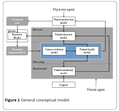
Figure 1: General conceptual model.

Psychosocial dimension: The psychological dimension includes an emotional model of the patient agent and its social influences, especially in the form of support from family members and nurses. This model describes a response to specific situations. This model will eventually contribute to measuring the patient quality of life during treatment.

Physiological dimension: This dimension includes both the patient’s health model (its general physical and health condition) and its cancer evolution model. Both are affected by treatment in different manners, while influencing each other. In practice, this dimension includes on the one hand, the absolute physiological state of the patient and cancer, and, on the other hand, the perception of this state obtained from observations (e.g., analysis, scans and biopsies). While the first information is not necessarily known, the second can be outdated, and more or less accurate. The variable describing the cancer evolution model in particular is described in the next section. Finally, in this model, the patient health model is influenced by his or her emotional model.

Decision dimension: This dimension includes both the patient’s and the physician’s decision models. It represents the main actors’ decision-making processes and preferences that contribute to treatment selection and treatment implementation. It is the part of the conceptual model that directly contributes to the decision and implementation of patient care trajectories. Here, the patient decision model is influenced by its health and emotional models, while the physician decision model is influenced by the patient cancer and health models. The patient decision model also contributes to plan each individual treatment according to the system resource availabilities.

System dimension: The system dimension represents the virtual hospital resources and processes. When a physician requests a type of treatment, it must be plan according to the hospital priority, the workload of the resources required for this kind of treatment, as well as the preferences of the patient.

The different sub-models of these dimensions influence each other in order to emulate the general relationships between the patient, his/her cancer, the medical staff, and the patient's support. The relationship between the patient and the hospital processes and resources are addressed through the dynamic specification of the treatment program into the care trajectories, which defines how the patient interacts with the different resources for his/her treatment and tests/scans. The next section focuses on the cancer evolution model and the link between cancer evolution and the physician decision model.

Cancer evolution model

Modeling the evolution of cancer is an important step for the simulation of care trajectories. In order to do this, the cancer will be modeled into two parts, the main tumor and metastases. Metastases are meant as a general term referring to every cancerous cell found in the patient’s body that is not part of the main tumor. This may be an isolated cell traveling in the patient's body or a small tumor hooked somewhere else than the main tumor. The main tumor size and the number of metastases are two important information as they influence the decision about the treatment [31]. Both will be simulated from their appearance (size 1 cell for the tumor and no metastasis) to the end of the treatment. It is useful to model the evolution of the cancer before the diagnosis so that out of treatment evolution parameters can be validated and the distribution of metastasis density can be known.

The evolution of the tumor model that will be described later has four parts: a free evolution and the three evolutions under each of the three treatments, which are radiation therapy, surgery and chemotherapy developments.

For the metastases evolution model, there are only two parts: as for the tumor model, a free evolution and an evolution under chemotherapy. There is no special evolution under radiation therapy because it has no effect on metastasis other than to reduce the emission of cancerous cells by the main tumor. If we neglect this impact, it is considered that they evolve in the same way as free evolution. Thus the only treatment affecting metastases is chemotherapy.

Tumor free growth

There is a lot of mathematical models of tumor growth based essentially on population-based models [32]. The original population-based model was developed by Maltus at the end of the 18e century, using equation 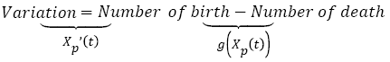(1):

(1)

Where Xp(t) is the tumor size over time given in numbers of cells. One of the most common formulas used for g(x) is an empirical law (see equation 2) described by Gompertz in 1825 [32], which describes the evolution of the main tumor from the appearance of the first cancerous cell to a larger tumor.

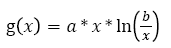(2)

With a being the rate of tumor growth (it is related to doubling time (DT) of the tumor); b is a constant equals 1012 and represents a maximum diameter of 12.4 cm (this value is used in most studies on solid tumors). Other tumor growth models exist, such as logistic and exponential models. The Gyllenberg-Webb model divides the evolution of the tumour in different phases depending on its size in order to describe its evolution more precisely [33].

In the simulation, the Gompertzian formula for the tumor free evolution was used. In order to determine a, we used which characterizes the tumor growth of 27 patients suffering from colorectal cancer [34]. Using this empirical study, we computed a Weibull distribution law of the doubling time, from which we randomly generated a doubling time DT. Assuming that this doubling time is a constant over the tumor growth, this allows us to calculate the time it takes for the tumor to be a given percentage P of the maximum size b using equation 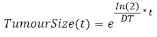[3].

(3)

Once the T is known, a is calculated using the Gompertz curve function, as shown in Figure 2.

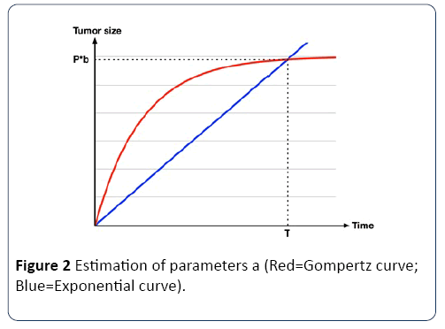
Figure 2: Estimation of parameters a (Red=Gompertz curve; Blue=Exponential curve).

Therefore, the link between the doubling time and a can be calculated using equation 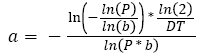(4).

(4)

Tumor growth after radiation therapy: First, only external radiation therapy is modeled. Its impact on the size of the tumor is calculated one session at a time. Consequently, the remaining number of cells is the number of cells before treatment multiplied by the percentage of surviving cells S represented by equation (5) from [3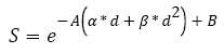5].

(5)

With α and β being constants for colon and colorectal cancer, respectively 0.339 and 0.067, as empirically estimated by Suwinski R, et al. [36]; d is the dose used during the session; and A and B are two parameters associated with the patient, corresponding to the effect of a variety of factors. They follow a normal distribution determined using [36]. This model is based on two assumptions. First, each cell that cannot further divide itself after the radiation therapy session is considered dead. Second, the tumor keeps growing freely between sessions.

Tumor growth during chemotherapy: The action of chemotherapy is determined using a model developed and tested with two types of chemotherapy drug (i.e., Fluorouracil and Capecitabine) on colon and colorectal cancer [37]. Based on this study, the function g(x) in equation (1) is described by equations (6) and (7):

(6)

(7)

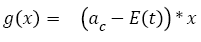
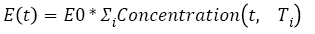
With ac being the exponential growth factor of the tumor. It is determined according to the parameters of the Gompertzien growth and the tumor size at the beginning of chemotherapy. Concentration (t,Ti) represents the function of drug concentration injected at time T during session i, in the patient’s body over time. E0 is the effect of the drug on the decrease of the tumour [32]. E0 depends on the patient and on the type of treatment. We model three types of drug administration: Oral, injection with syringe and long injection like Portacaths [38] and Piccline [39]. The function of concentration of drug in the patient’s body over time is different for these three types of administration (see equations 8, 9 and 10) [32,37].

For injection with syringe and oral administration:

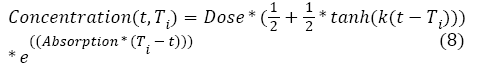
With Absorption being the speed of drug elimination from the patient’s body; k is the speed of drug assimilation; and Dose is the dose injected during the session. The only different between injection with syringe and oral administration is k, which is bigger for injection (Figure 3).

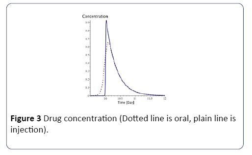
Figure 3: Drug concentration (Dotted line is oral, plain line is injection).

For long injection: Concerning long injection, the only new parameter is duration, which is the length of time of the injection, as shown in equation (9), and Figure 4.

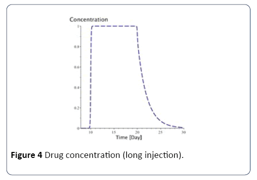
Figure 4: Drug concentration (long injection).

Finally, the function of the tumor’s size during chemotherapy is:

(10)

With STc is the tumor’s size before the beginning of chemotherapy. This value is also used in the metastatic evolution model.

Tumor growth after surgery: The effect of surgery on the size of the tumor is simpler than the other two treatments described above. Indeed, depending on the cancer (colon or rectum) and the type of surgery, the effect of the surgery can be described as a probability of having cancerous cells from the main tumor remaining in the body. The next section presents an illustrative example of a cancer patient treated with two treatments.

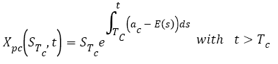
Illustrative example: In order to illustrate the evolution of a main tumor, before, during and after treatment, this example, shown in Figure 5, shows the tumor’s diameter in mm over time. First, there is a three-year evolution phase before any treatment. Then, there are three weeks with 5 radiation therapy sessions per week, followed by one week of rest, and finally six months of chemotherapy.

Figure 5: Tumor’s diameter in mm over time.

Metastases growth

For the development of metastases, we use a model developed by Iwata [40]. In this model, the growth of main tumor and the metastases are described by a set of mathematical equations. The tumor growth is modeled by Xp(t), which can either be the Gompertzian function (2) or the exponential function (3). Next metastases growth, produced by the main tumor and other metastases, is described by equation (11).

(11)

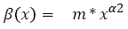
With m being the coefficient of colonization, and α2 being the fractal dimension of blood vessels infiltrating the tumor. In turn, as shown in Figure 6, new tumors grow according to Xp(t) and produce cancerous cells according to β(x).

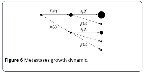
Figure 6: Metastases growth dynamic.

Considering that all tumours evolve similarly is not entirely correct. Indeed, although they all originate from the main tumour (i.e., their nature is similar), their spread and evolution depend on their location. However, accurately modeled movement of each tumour cell in the body is impossible. The Iwata model and its assumptions are considered valid and used in the majority of evolution models of metastases. Iwata’s model is defined by the system of equation 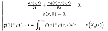(12):

(12)

With ρ(x,t) being the density of metastases in the patient's body (i.e., the number of tumours containing x cells at time t), and g(x) being the function. Both parameters m and α2 are specific to each patient and have a normal distribution, which are determined [31,40].

The value of interest for the decision-making is the Metastatic Index (MIn). It is defined by equation (13) [31]. It represents the total number of metastatic tumors of size between n and Xp(t) in the patient's body at time T.

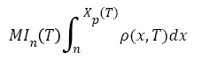(13)

The resolution of the Iwata model is more complex than that of the primary tumor. Furthermore, there is general solution of this model with a function g(x) with chemotherapy. Therefore, in order to keep calculation time reasonable within the simulation environment, the Iwata model is only used to describe the evolution of metastases without treatment using function g(x) defined in equation (2).

Metastases growth during chemotherapy: Granted there is no general solution to the Iwata model with chemotherapy, in order to determine the effects of chemotherapy on metastases, we first made three assumptions:

1. Cancer cell dispersion in the body (i.e., β(x)) is neglected. Because cancer cell progressing through the patient's body is directly in contact with the drug, we assume it is automatically destroyed.

2. All metastatic tumors evolve along the same decay law as the primary tumour under chemotherapy. In this study, we use equation (6).

3. The number of tumors given by ρ(x,Tc), as defined in equation (12) at the end of the free evolution of metastases, remains unchanged during the chemotherapy treatment. Only the tumor’s size is affected.

Based on these hypothesis, the new distribution of metastases during chemotherapy (t>Tc) can be calculated based on ρ(x,Tc) as defined at the end of the free evolution of metastases, using equation (14):

(14)

We define a new function Xpc-1 as.

(15)

Therefore, MI during chemotherapy can be calculated using equation 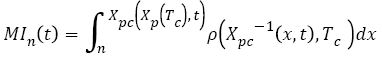(16):

(16)

Model integration

Each of these individual models describes part of the entire cancer evolution with and without treatment. For the purpose of building a simulation model, they must be integrated. However, they are continuity gaps at the interface of each model that require some adjustments. More specifically, because the Iwata model is difficult to solve when initial conditions are changed (e.g., after a chemotherapy session), we made hypothesis in order to simplify the integration of the different models.

First, between surgery and chemotherapy, the primary tumor does not produce metastases because it has been removed. However, an opposite effect occurs after the removal of the main tumor favoring metastases development through angiogenesis [41]. Therefore, because we do not know which effect is dominant, the metastases growth model proposed and it is used after surgery.

Similarly, concerning radiation therapy, the decreased metastases production by the main tumor is neglected. Indeed, at this stage of the cancer, the production of metastasis is partly due to metastases themselves [42]. Furthermore, for staging, as seen in the next section, we only consider metastatic tumors of size greater than 5X106 cells. Consequently, this effect has little impact on metastases of this size, because metastatic cells produced during radiation therapy do not have enough time to growth bigger than this size before chemotherapy.

Next, between consecutive chemotherapy sessions, or during chemotherapy breaks due to fatigue of the patient, we assume that the E(t), which defines the impact of chemotherapy drug in the tumor growth model during chemotherapy (i.e., equation (7)), is equal to zero until the next session due to a lack of drug in the body. Therefore, we model the tumor growth between sessions as exponential (i.e., equation (3)), because it is sufficiently accurate for short period of time (the difference between the gompterz and exponential growth over three weeks is less than 0.5% in most cases). However, note that the gompterz growth was used for the evolution of the tumor over the large period before any treatment. In order to calculate the parameter ac (from equation (6)), we used the technic.

Another challenge, for the integration these models, lies in the calculation of the metastatic index (MI). Indeed, the upper limit of the integral (equation (15)) is the tumor size during free evolution. However, during a treatment, the upper limit is no longer equal to the size of the tumor. For example, during radiation treatment, the tumor size decreases a lot, although the treatment has no direct impact on metastases. Therefore, the tumor size after radiotherapy cannot be taken as the upper limit of the integral. To solve this problem, we take as an upper bound the fictitious tumor size corresponding to its free evolution. For chemotherapy treatment, the upper bound is also the size of the fictitious tumor, which evolution is described by the evolution of the tumor with the chemotherapy model.

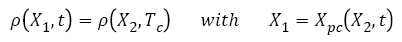
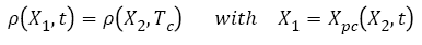
Cancer observed state and actual state

The physician’s decision on which treatment to be performed on the patient is not based on the output values of the mathematical models presented above, which represent a simulation of the actual state of the cancer that can never be completely known. Instead, treatment decisions, which will eventually be simulated as well, are based on criteria such as TNM staging of cancer [43]. TNM staging can be considered as the observed state of the cancer. Consequently, we must link both the observed state and the actual state in order to be able to define what treatment to perform for each patient. In the simulation environment, TNM staging is only determined before deciding which treatment to follow during treatment, physicians are more interested by the reactions of the cancer and the general health of the patient in order to interrupt or adjust the treatment. The NCCN Guideline explains the TNM staging for colorectal cancer in details. However, for simplification purpose, this staging was adjusted, as described [44]. Here, T only corresponds to the general stages of cancer (i.e., 1, 2, 3 or 4), while N and M are Boolean variables specifying respectively if there are or not metastases lymph node (i.e., N), and if there are or not distant metastasis (i.e., M). This simplified staging identifies the most important aspect to know for treatment decision, using the NCCN guideline.

Tumor: The output of the tumor model is its size given in numbers of cells. In order to convert the number of cells into the diameter of the tumor, we assume that 1 mm3=106 cells, as explained and that the tumor is a sphere [43,44]. With these assumptions, the conversion can be done using equation 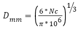(17).

(17)

Where Nc is the number of cells in the tumor.

In the TNM classification, T corresponds to the penetration of the tumor through the various tissue layers of the colon and not directly to the tumor size [45]. However, it is possible to estimate the tumor penetration distributions according to its tumor size, as shown in Figure 7 [46,47].

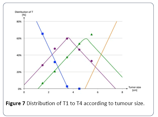
Figure 7: Distribution of T1 to T4 according to tumour size.

Therefore, from the size of the tumor given by the mathematical model, a probability of belonging to a particular penetration (i.e., T1 to T4) is determined. For example, a tumor with a 4-centimetre diameter has a 45% chance of being a type T3 penetration, and a 55% chance of being a type T2 penetration.

Nodes and metastases: In order to determine M, the same method was applied. If IM108 is greater than 1 at the time of diagnosis, we consider that the patient has metastases in at least one organ and his M is equal to one [31]. Concerning N, we proceed similarly. However but we use IM5X106 instead of IM108 because a size of 5X106 cells corresponds to 2.1 mm, which is the difference between the average size of the tumorfree lymph nodes and the average size of lymph nodes with metastatic infiltration, measured [48]. Furthermore, below this size, there is very little chance that the analysis of nodules comes out positive for the presence of cancerous cells [31].

Clinical pathways module

In this section we performed a critical analysis on the existing pathways provided by NCCN guidelines version 2015 (www.nccn.org) and Cancer Care Ontario (www.cancercare.on.ca) treatment pathways and further we consulted with the medical staff at JGH to develop a platform for the clinical pathways associated with the type of cancer (colon or rectal) and the different stage of cancer to be incorporated into the simulation. In addition, we also reviewed a demo database acquired from JGH on colorectal cancer patients entering the system in 2013, to analyze and identify the dissimilarities for the year of 2013.

Colon cancer pathways: The treatment of colon cancer depends on the stage, location of the tumor and the overall health of the patient. Surgery and chemotherapy are two currents treatments of colon cancer. After reviewing the pathology reports (imaging, polypectomy or biopsy) and staging the cancer, surgeon decides whether the patient is a candidate for resection surgery or medically unfit for surgery. If operable, the patient is scheduled for colectomy with Enbloc Removal of Regional Lymph nodes; if not operable the patient is instructed for palliative chemotherapy or radiation therapy after consulting with medical oncologist. Post-operation recovery period for patients with colon cancer is usually 4-8 weeks.

Patients in Stage II are categorized as either low-risk or highrisk. Low risk stage II patients proceed to the cancer follow-up care pathway, however the high risk stage II patients with completely resected colon cancer are referred to medical oncologist and are considered for sessions of adjuvant chemotherapy and then proceed to cancer follow-up care pathway. Recommended chemotherapy protocols by Cancer Ontario and NCCN to the use of chemotherapy in Stage II high risk patient’s remains controversial (Figure 8).

Figure 8: Stage 1, 2, 3, 4 colon cancer treatment plan.

All stage III patients with completely resected colon cancer are referred to medical oncologist for adjuvant chemotherapy. If surgery unsuccessful the surgeon might consider reresection. With or without resection the patients are referred to medical oncologist to be considered for chemotherapy.

Patients in Stage IV are first considered for colon resection if and only if there is an imminent risk of destruction or significant bleeding. In case the liver and/or lung metastases exist and are resectable, the patient is either directly considered for staged resection of metastatic and colon cancer or is firstly referred to medical oncologist for neoadjuvant chemotherapy and then is scheduled for surgery. After the surgery the patient is considered for adjuvant chemotherapy.

If the liver and/or lung metastases are potentially resectable, firstly the patient proceeds to chemotherapy. After the chemotherapy treatment, the patient is re-evaluated for resctablility, if resectable, the patient is scheduled for staged resection of metastatic and colon cancer.

Various pathways were observed in this stage. Pathways such as Radiotherapy and chemotherapy protocols, before and after resection and in some cases combinations of radiotherapy and chemotherapy protocols were also observed.

Colorectal cancer pathways: After reviewing the pathology report (polypectomy or biopsy) and staging the cancer, the surgeon decides whether the patient is a candidate for resection surgery or medically unfit for surgery. After surgery the patient is referred to Pathology for further screening tests. If not operable the patient is instructed for palliative chemotherapy or radiation therapy after consulting with a medical oncologist. Post operation recovery period for patients with colorectal cancer is usually 6-8 weeks. After searching the medical databases and consulting with surgeons at JGH we realized that even though the treatment recommended by NCCN and Cancer Ontario is resection in the case of stage I cancer, many believe radiotherapy alone is successful in removing the cancerous cells (Figure 9).

Figure 9: Stage 1, 2, 3, 4 colorectal cancer treatment plan.

For the stage II and III, the surgeon needs to decide whether the cancer is resectable or not. If resectable, the patient is referred to a radiation oncologist and a medical oncologist for preoperative therapy which includes preoperative chemoradiotherapy or preoperative hypo fractionated radiotherapy alone. After preoperative therapy the patient is scheduled for resection surgery the patient is then referred to pathology for further tests and thereafter to adjuvant chemotherapy if necessary. However, if the cancer is not resectable, the possibility for down-staging the cancer with chemoradiotherapy is assessed. If possible, the patient is referred for chemo-radiotherapy while being re-evaluated for resectability by allowing adequate time for down-staging. If down-staged the patient is then scheduled for surgery, however if downstaging is not successful, the patient is instructed palliative chemotherapy. If there is no possibility for down-staging the cancer with chemo-radiotherapy the patient is instructed for palliative radiation with or without chemotherapy.

For patients in stage IV of rectal cancer, the respectability of the primary tumor and of metastatic disease is first evaluated. Subsequently, a multidisciplinary team of surgeons, radiation oncologists and medical oncologists create an individualized care plan for the patient. If the primary tumor is resectable and the metastatic disease is resectable or potentially resectable, a neoadjuvant chemo-radiotherapy plan is formed for the patient. After the therapy, the patient is scheduled for the resection of the primary tumor. Afterwards neoadjuvant therapy is prescribed. After the chemotherapy metastatic lesions are assessed and if possible the patient is scheduled for resection of metastatic liver lesion. If the metastatic disease is not resectable the patient is instructed for appropriate palliative therapy. However if primary tumor is not resectable, neoadjuvant chemotherapy is considered for down-staging and converting the tumor to a resectable one. If down-staging is successful the patient follows the aforementioned pathway, However if down-staging is not successful the patient is instructed for appropriate palliative therapy.

Model Validation

In order to validate the model, we carried out two experiments, using our simulation platform (based in the JADE Platform) with a 3,5 GHz Intel Core i7 processor and 32 Go of RAM. The first experiment aims at assessing the ability of the model to replicate the results of different clinical studies with specific treatment protocols. The second experiment extends the first by assessing the ability of the model to interpolate the results of several clinical studies with different treatments (i.e., different dosage, different protocols, and different treatment duration). In other words, this second experiment aims at analyzing the ability of the model to estimate the outcome of treatments for which we do not have clinical studies.

In both experiments, in order to compare the simulation results with actual data, we used the standard classification criteria of the World Health Organization which are also used in the clinical studies used for validation [49]. This classification distinguishes patients according to the cancer response (i.e., partial response (PR); complete response (CR); stable disease (SD); and progressive disease (PD)). Due to the limits of our model, which does not currently take into account patient mortality, it was not possible to consider other criteria such as the overall survival (OS), the disease free survival (DFS) and the progression free survival (PFS).

In practice, this classification is based on the evolution of the size of the tumours. More specifically, practitioners calculate the sum of the products of the greatest perpendicular diameters (SPD) of the measurable metastases, which is a measure of an area, and analyze their evolution between observations. However, in our model, we can approximate the sum of the volume of tumours using Equation (18).

(18)

With n being the minimal size of tumors to be included (in number of cells).

Therefore, because our model returns a number of cells, which is a proxy of the tumor’s volume, we converted the threshold value of each class based on the volume a sphere and the area of the disk . For example, Partial Response (PR) is defined as a SPD reduction larger or equal to 50%, which corresponds to a decrease of at least 64.65% in the total number of metastatic cells. Concerning complete response (i.e., CR), a patient is considered with a complete response if his or her , which mean that all metastases of at least 108 cells are gone.

Finally, in order to measure the performance of the calibration and the capacity of the model to replicate the results of clinical studies, we used the average Euclidean distance between the simulation results and the clinical studies, as calculated with equation (19).

(19)

First experiment

In this first experiment, we must first calibrate the model’s parameters. In order to do so, we use data from six clinical studies which allows us to validate our metastases growth model during chemotherapy treatment [50-60]. Indeed, as it is the least documented and modeled part of the cancer evolution, we prioritize the validation of this part of the model. The data from these clinical studies includes the stage of the cancer, the method of patient selection and the protocol of treatment received by patients for Capecitabine chemotherapy. The first study tested two administration protocols (i.e., a and b) on a sample of 35 and 40 patients. The other studies tested only the first protocol (i.e., a) on a sample of 42 patients, 301 patients, 32 patients, 96 patients and 51 patients. Patients in the protocol a received two daily doses from day 1 to 14, followed by a period of rest (day 15 until 21), and followed by a new treatment cycle starting on day 22. Patients in the protocol b received two daily doses continuously without rest periods. The model was calibrated for these two administrations protocols and for both sample sizes.

Selection of the virtual population: For each protocol/ population we aim to replicate, we must first create several populations of virtual patients. To do so, it is not possible to simply create a virtual population with similar statistics as the real population. Indeed, the metastases distribution is correlated with the characteristics of the primary tumor because they share parameters. Therefore, we have to simulate all virtual patients starting at T0, when the first cancer cell appears. Subsequently, we determine two dates per patient, T1 and T2, respectively, when the tumor size falls within the range of interest, as defined by the studies, and when it comes out of this range. The date of diagnosis Td is selected randomly between T1 and T2, as shown in the Figure 10.

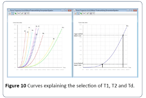
Figure 10: Curves explaining the selection of T1, T2 and Td.

Once the diagnosis date is fixed, we determine the stage of the patient. From this large population of virtual patients, we select those whose characteristics are similar to the actual population to create our population test. Thus the total number of virtual patients is known in advance and it is necessary to initially simulate a large number of patients to have a sufficiently large test population. In order to select a virtual population similar to the actual populations selected in clinical trials in the first experiment below we took patients with stage 4 and with MI5*108 greater than 1, which corresponds to metastasis larger than 10 mm [50-60].Calibration: In order to calibrate the model for the configurations of the six clinical studies, we first need to estimate the impact of each parameter on the results based on their role in the model. For example, the percentage of progressive disease is only defined by the parameter of the Gompterz evolution a and the parameters of the chemotherapy E0, Absorption and Dose. Other parameters such as m, α and the maximum and minimum size of the tumor in the selection of the virtual population only affects the distribution of patients in the three categories: CR, PR and SD.

Thus, to calibrate the model, we proceed by try-and-error, using a dichotomy approach to set each parameter and replicate the results of the clinical studies as best as possible (Table 1).

Table 1 Calibration results.

	Study 1 Protocol b	Study 1 Protocol a	Study 2 Protocol a	Study 3 Protocol a	Study 4 Protocol a	Study 5 Protocol a	Study 6  Protocol a
Parameters	Average(Standard deviation)	Average(Standard deviation)	Average(Standard deviation)	Average(Standard deviation)	Average(Standard deviation)	Average(Standard deviation)	Average(Standard deviation)
M	6 *10-8 (3*10-9)	6 *10-8 (3*10-9)	6 *10-8 (3*10-9)	6 *10-8 (3*10-9)	6 *10-8 (3*10-9)	6 *10-8 (3*10-9)	6 *10-8 (3*10-9)
α2	0,66 (0,03)	0,66 (0,03)	0,66 (0,03)	0,66 (0,03)	0,66 (0,03)	0,66 (0,03)	0,66 (0,03)
P	0,87	0,87	0,87	0,87	0,87	0,87	0,87
Lower Limit	5	5	5	8	8	8	8
Upper Limit	45	45	45	60	60	60	60
E0	3,4*10-3	1,68*10-3	1,68*10-3	1,68*10-3	1,68*10-3	1,68*10-3	1,68*10-3
Absorption	0,87	0,87	0,87	0,87	0,87	0,87	0,87
Dose	0,732	1,25	1	1,25	1,25	1	1,25
Stage	II	II	II	III	III	III	III
Patients Number	40	35	42	301	302	96	51
Chemotherapy duration	109	109	126	147	123	231	42

Simulation results: Different simulation tests were carried out for each set of parameters. In all tests, the virtual population samples were, like for calibration, different in size to those of the six studies. In other words, protocol b of study 1 was tested with samples of 40 patients, protocol a of study 1 was tested with samples of 35 patients and protocol a was tested by five studies (2 to 6). The model results of the simulation tests are consistent with the results of the studies, and our model can adequately reproduce reality. Figure 11 describes the average value of E of the simulation tests for each experiment.

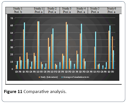
Figure 11: Comparative analysis.

Concerning the duration of the simulated treatments, the median duration reported in both studies was used for the corresponding tests. The dose of chemotherapy was considered constant throughout the treatment. Because our model does not take into account side effects and patients mortality rate, we adjusted the results of clinical studies to remove these cases for comparison purpose. The final values of the parameters for each calibration are shown in Table 2. Concerning the parameter Absorption, it has been set equal to its defined value, while the average value of α2 was taken [32,40].

Table 2 Comparative analysis and euclidian distance.

		Study (Literature)	Average of simulation tests
Study 1 Protocol b	CR	5,38	10,80,556
	PR	17,2	11,888889
	SD	54,84	63,80,556
	PD	22,58	13,5
Study 1 Protocol a	CR	3,16	10,02,778
	PR	22,11	1,81,111
	SD	65,26	65,25
	PD	9,47	66,11,111
Study 2 Protocol a	CR	2	75,83,333
	PR	43	30,88,889
	SD	48	56,02,778
	PD	7	5,5
Study 3 Protocol a	CR	0,34	9,40,484
	PR	21,06	18,29,677
	SD	64,33	61,16,129
	PD	14,27	1,11,371
Study 4 Protocol a	CR	0,3	70,17,742
	PR	25,5	2,05,871
	SD	49	61,96,774
	PD	14,2	10,42,742
Study 5 Protocol a	CR	55 (CR + PR)	40,92742 (CR + PR)
	PR
	SD	31	51,80,645
	PD	6	72,66,129
Study 6 Protocol a	CR	0	4,99,026
	PR	2	93,74,411
	SD	53	59,63,712
	PD	45	25,99,821

Discussion

The calibration was more difficult in the cases of clinical test with small population sample. This difficulty can come from several reasons. First, the small number of patients tested can cause an inhomogeneous population. Similarly, random number generation can also affect the distribution of the population with such small size. Next, the relative inaccuracy of the model may be too large with such small patient populations, which may lead to results that are more significantly different from actual data.

In addition, it is interesting to note that the set of parameters to reach accurate results is not unique. Indeed, it was possible to find another set of parameters (Table 3) with a value of Absorption equal to 0.4, while keeping the others parameters within the acceptable boundary, which also gave a good calibration for the protocol a of the study 1. Indeed, E was equal to 3,5 and here it is the new set of parameter:

Table 3 Second set of parameters for protocol a study 1.

Protocol a Study 1
Parameters	Average(Standard deviation)
M	6*10-8 (1*10-9)
α2	0,66(0,01)
P	0,004
Lower Limit	34
Upper Limit	34
Dose	1,25
E0	1,13E-03
Absorption	0,4

The parameters of Protocol a of studies 1 and 2 are similar and it is possible to use the parameters of one to simulate the other with E<7 for 2 from study 1 and E <4.5 for 1 from study 2. Unfortunately, using the parameters of one protocol to simulate the other has not given good results. This may be due in part to the simplifications we introduced in order to simulate these protocols. Indeed, we made two assumptions. The first was to consider a constant dose for all patients during the entire treatment. This assumption is correct insofar as both studies administered at least 90% of the planned dose. However, the second assumption was to take the same treatment duration for all patients matching the median treatment duration recorded in the clinical studies. Unfortunately, in practice, treatment duration varies greatly from one patient to another, especially due to the side effects and patient's response. Consequently, a second phase of validation will be performed with more specific data for each patient from the Montreal Jewish General Hospital.

Finally, once model calibration is extensively tested with several protocols, it could eventually be used to simulate the outcome of various treatments and protocols for specific patients, and thus, serves as a medical decision support system. Indeed, with some medical tests it would be possible to estimate parameters a, m and α2 of the patient within a certain margin of error. For instance, a could be approximated using two imaging tests of the primary tumor to determine its size at two different dates. m and α2 could be determined by estimating the mass of visible metastases using imaging, which should be equal to the one given by the Iwata model at the same tumor’s size and time of diagnosis. Using these estimated parameters, the outcome of a treatment for a patient could be simulated with specific statistical distributions for the unknown parameters, which would then give probable outcomes for that patient.

Second experiment

In this experiment, we aim at assessing the capacity of the model to interpolate the results of clinical studies with different treatments, such as different dosage, different protocols, and different treatment durations. To do so, we used another set of studies conducted with another type of chemotherapy used in colon and colorectal cancer, the 5- fluorouracil (5-FU), which is well documented in the literature. In particular, we used which regroup a number of clinical studies on 5-FU, in order to define the response (CR + PR) as a function of the average dose per time unit (for one cycle of chemotherapy), using linear regression (Figure 12) [52].

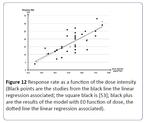
Figure 12: Response rate as a function of the dose intensity (Black points are the studies from the black line the linear regression associated; the square black is [53]; black plus are the results of the model with E0 function of dose, the dotted line the linear regression associated).

First, we calibrated the model using with E=1.06 [53]. The protocol targeted in this study is 5 day of 5-FU repeat every four weeks. Once calibrated, we varied the dose (all other parameters being unchanged). As see in Figure 12, that the variation of the dose in the model has a greater impact than in reality. In order to adjust this, we assumed that parameter E0, which describes the effect of the drug on the decrease of the tumor, should be a function of the dose. Therefore, in order to adjust the impact of the dose, we introduced a new E0, as a function of dose (Equation 20):

(20)

Once a and b were calibrated, the new results presented in Figure 12, an excellent capacity of the model to interpolate the impact of the dose.

Similarly, we also tested the capacity of the model to interpolate the impact the total treatment duration. Once again, the impact of the treatment duration was more significant than in reality. However, we were not able to find a simple mathematical function capable of taking the impact of treatment duration into account. We suspect that E0 must either be a function of the total treatment duration, or must change in time during treatment as if some sort of mechanism would affect the capacity of the drug to decrease tumor size. However, because the time of treatment described in the literature, when available, is only an average, it is difficult to properly define E0 with the data available. This must be done with more specific data.

Conclusion and Future Work

This paper introduced a conceptual model aiming at the development of a simulation environment capable of emulating the simultaneous care trajectories of several of cancer patients. More specifically, this paper introduces a cancer evolution model, which is the first developmental step of such a simulation environment.

Before this model can be implemented and tested within the simulation environment, several other aspects of the conceptual model presented in Figure 1 will have to be developed. Along the same line, the hospital resources and management processes will have to be modeled as well. But one of the first things to do before its integration into the simulation platform will be to validate the entire model with actual data from the hospital.

Once completed, the configuration of the many agents of this simulation platform will be adjusted in order to emulate accurately reality. This paper shows that preliminary results indicate that it is possible to develop such a model, although development and analysis are required.

The validation of the entire simulation environment with respect to actually data for a hospital will be part of an extensive aspect of the project. Once validated, this simulation environment will be used by the hospital in order to evaluate the benefits of specific organizational changes to both the hospital performance and the patients’ quality of life.

Concerning the development of the simulation platform, the next step is be to calibrate and test this model with other chemotherapies and treatment protocols with specific patient data. However, there is still much work to do to improve this overall model. For instance, one general improvement concerns the modeling of the combined effects of radiation and chemotherapy administered simultaneously. Another important aspect concerns the modeling of the interactions between cancer treatments and the treatments of other health issues (i.e., co-morbidity).

Concerning the modeling of new treatment, the second should also be adapted to include the impact of internal radiation therapy (i.e., brachytherapy) as it is more and more used in hospitals. Moreover, it would also be useful to take into account the interactions between the different treatments as surgery impacts metastasis angiogenesis, which makes metastasis grow faster [41]. In addition, long-term effects of treatment should be integrated as the tumor may take some time to regrow after radiation therapy. However, these effects are often random and causes for their presence or absence are unknown, making them difficult to model. Eventually, the model must also include mortality and its expected step for any medium term following work. This should be easy insofar as mortality models based on the evolution of cancer already exist [54,55].

Along the same line, the model must also include side effects because they are important causes of resource utilization variability between patients, as well as indicators of patient quality of life.

Finally, this model of cancer colon and colorectal evolution is easily adaptable to other type of carcinoma cancer [56], because the equation used was made for general cancer and not only for the colon and colorectal. For example, Iwata use his model on liver cancer.

21413

References

1. Heath B, Hill R, Ciarallo F (2009) A survey of agent-based modeling practices. ‎J Artif Soc Soc Simul12: 9.
2. Michel F, Ferber J, Drogoul A (2009) Multi-Agent systems and simulation: A survey from the agents community's perspective, multi-agent systems: simulation & applications.
3. Treuil JP, Drogoul A, Zucker JD (2008) Modélisation et simulation à based agents, Exemples commentés, outils informatiques et questions théoriques. Dunod.
4. Jones B, Dale RG (2000) Radiobiological modeling and clinical trials. Int J Radiat Oncol Biol Phys48: 259-265.
5. Mustafee N, Katsaliaki K, Taylor SJE (2010) Profiling literature in healthcare simulation. Simulation 86: 543-558.
6. Jun J, Jacobson S, Swisher J (1999) Application of discrete-event simulation in health care clinics: A survey. ‎J Oper Res Soc 50: 109-123.
7. Fone D, Hollinghurst S, Temple M, Round A, Lester N, et al. (2003) Systematic review of the use and value of computer simulation modelling in population health and health care delivery.J Public Health Med25: 325-335.
8. Roberts SD (2011) Tutorial on the simulation of healthcare systems. InProceedings of the Winter Simulation Conference. pp: 1408-1419.
9. Stainsby H, Taboada M, Luque E (2009) Towards an agent-based simulation of hospital emergency departments. In:SCC 2009-2009 IEEE International Conference on Services Computing, IEEE Computer Society, Bangalore, India. pp: 536-539.
10. Knight VA, Williams JE, Reynolds I (2012) Modelling patient choice in healthcare systems: Development and application of a discrete event simulation with agent-based decision making.J Simul6: 92-102.
11. Figueredo GP, Aickelin U (2011) Comparing system dynamics and agent-based simulation for tumor growth and its interactions with effector cells.In Proceedings of the 2011 Summer Computer Simulation Conference,Society for Modeling & Simulation International. pp: 52-59.
12. Jennings NR, Sycara K, Wooldridge M (1998) A roadmap of agent research and development. Autonomous agents and multi-agent systems 1: 17-38.
13. Wooldridge M, Jennings NR (1995) Intelligent agents: Theory and practice. Knowledge Eng Rev10: 115-152.
14. Chaib-Draa B, Jarras I, Moulin B (2001) Multi-agent systems: general principles and applications. Hermès Edition.
15. Franklin S, Graesser A (1997) Is it an Agent, or just a Program?: A Taxonomy for Autonomous Agents, in Intelligent agents III agent theories, architectures, and languages. Springer, Germany. pp:21-35.
16. Nwana HS (1996) Software agents: An overview. Knowledge Eng Rev 11: 205-224.
17. Briot JP, Demazeau Y (2001) Principles and architecture of multi-agent systems (Treaty IC2, Computer and Information Systems), Hermès Lavoisier.
18. Nealon J, Moreno A (2003) Agent-based applications in health care, in Applications of software agent technology in the health care domain. Springer, Germany. pp: 3-18.
19. Devi MS, Mago V (2005) Multi-agent model for Indian rural health care. Leadership in Health Services 18: 1-11.
20. Kanagarajah A, Parker D, Xu H (2010) Health care supply networks in tightly and loosely coupled structures: Exploration using agent-based modelling. Int J Systems Sci 41: 261-270.
21. Wang L (2009) An agent-based simulation for workflow in emergency department. Systems and Information Engineering Design Symposium. pp: 19-23.
22. Aringhieri R (2010) An integrated DE and AB simulation model for EMS management.In 2010 IEEE Workshop on Health Care Management, WHCM 2010, Venice, Italy; 2010. IEEE Computer Society.
23. Laskowski M, McLeod RD, Friesen MR, Podaima BW, Alfa AS (2009) Models of emergency departments for reducing patient waiting times. PLOS One 4: e6127.
24. Jones SS, Evans RS (2008) An agent based simulation tool for scheduling emergency department physicians.AMIA Annual Symposium Proceedings. American Medical Informatics Association2008: 338-342.
25. Zhang W, Yao Z (2010) A reformed lattice gas model and its application in the simulation of evacuation in hospital fire.  IEEE International Conference on Industrial Engineering and Engineering Management, IEEM2010, 2010, Macao, China.pp: 1543-1547.
26. Krizmaric M, Zmauc T, Micetic-Turk D, Stiglic G, Kokol P (2005) Time allocation simulation model of clean and dirty pathways in hospital environment.In Computer-Based Medical Systems. pp: 123-127.
27. Paranjape R, Gill S (2010) Agent-based simulation of healthcare for Type II diabetes.In 2ndInternational Conference on Advances in System Simulation, SIMUL 2010, Nice, France; IEEE Computer Society.pp: 22-27.
28. Day TE, Ravi N, Xian H, Brugh A (2013) An agent-based modeling template for a cohort of veterans with diabetic retinopathy. PLoS One 8: e66812.
29. Barbolosi D, André F, Thompson AM, Laurentiis M, Esposito A, et al. (2011) Modeling of the risk of metastatic evolution in patients suspected of having localized disease.Oncology 13: 528-533.
30. Verga F (2010) Mathematical modeling of metastatic processes.University of Provence-Aix-Marseille.
31. Gyllenberg M, Webb GF (1988) Quiescence as an explanation of Gompertzian tumor growth. Growth Dev Aging 53: 25-33.
32. Bolin S, Nilsson E, Sjödahl R (1983) Carcinoma of the colon and rectum-growth rate. Annals of surgery 198: 151.
33. Wang P, Feng Y (2013) A mathematical model of tumor volume changes during radiotherapy. The Scientific World J 2013: 1-5.
34. Suwinski R, Wzietek I, Tarnawski R, Namysl-Kaletka A, Kryj M et al. (2007) Moderately low alpha/beta ratio for rectal cancer may best explain the outcome of three fractionation schedules of preoperative radiotherapy.Int J Radiat Oncol Biol Phys 69: 793-799.
35. Claret L, Girard P, Hoff PM, Van Cutsem E, Zuideveld KP, et al. (2009) Model-based prediction of phase III overall survival in colorectal cancer on the basis of phase II tumor dynamics.J Clin Oncol 27: 4103-4108.
36. https://www.cancer.ca/en/cancer-information/diagnosis-and-treatment/tests-and-procedures/subcutaneous-port/?region=on
37. https://www.cancer.ca/en/cancer-information/diagnosis-and-treatment/tests-and-procedures/peripherally-inserted-central-catheter/?region=on
38. Iwata K, Kawasaki K, Shigesada N (2000) A dynamical model for the growth and size distribution of multiple metastatic tumors. J Theoretical Biol 203: 177-186.
39. Peeters CF, de Geus LF, Westphal JR, de Waal RM, Ruiter DJ, et al. (2005) Decrease in circulating anti-angiogenic factors (angiostatin and endostatin) after surgical removal of primary colorectal carcinoma coincides with increased metabolic activity of liver metastases. Surgery137: 246-249.
40. Barbolosi D, Benabdallah A, Hubert F, Verga F (2009) Mathematical and numerical analysis for a model of growing metastatic tumors. Math Biosci 218: 1-14.
41. Akanuma A (1978) Parameter analysis of Gompertzian function growth model in clinical tumors. European J Cancer 14: 681-688.
42. Koscielny S, Tubiana M, Lê MG, Valleron AJ, Mouriesse H, et al. (1984) Breast cancer: relationship between the size of the primary tumor and the probability of metastatic dissemination. British J Cancer 49: 709.
43. https://www.e-cancer.fr/cancerinfo/les-cancers/cancers-du-colon/les-stades-du-cancer-colorectal
44. Brodsky JT, Richard GK, Cohen AM, Minsky BD (1992) Variables correlated with the risk of lymph node metastasis in early rectal cancer. Cancer69: 322-326.
45. Wolmark N, Fisher ER, Wieand HS, Fisher B (1984) The relationship of depth of penetration and tumor size to the number of positive nodes in Dukes C colorectal cancer. Cancer 53: 2707-2712.
46. Mönig SP, Baldus SE, Zirbes TK, Schröder W, Lindemann DG, et al. (1999) Lymph node size and metastatic infiltration in colon cancer. Ann Surg Oncol 6: 579-581.
47. World Health Organization (1979) WHO handbook for reporting results of cancer treatment.WHO, Geneva.
48. Van Cutsem E, Twelves C, Cassidy J, Allman D, Bajetta E, et al. (2001) Oral capecitabine compared with intravenous fluorouracil plus leucovorin in patients with metastatic colorectal cancer: results of a large phase III study. J Clin Oncol 9: 4097-4106.
49. Van Cutsem E, Findlay M, Osterwalder B, Kocha W, Dalley D, et al. (2000) Capecitabine, an oral fluoropyrimidine carbamate with substantial activity in advanced colorectal cancer: results of a randomized phase II study. J Clin Oncol 18: 1337-1345.
50. Hryniuk WM, Figueredo A, Goodyear M (1987) Applications of dose intensity to problems in chemotherapy of breast and colorectal cancer. Semin Oncol 14: 3-11.
51. Doroshow JH, Multhauf P, Leong L, Margolin K, Litchfield T, et al. (1990) Prospective randomized comparison of fluorouracil versus fluorouracil and high-dose continuous infusion leucovorin calcium for the treatment of advanced measurable colorectal cancer in patients previously unexposed to chemotherapy. J Clin Oncol 8: 491-501.
52. Heun JM, Grothey A, Branda ME, Goldberg RM, Sargent DJ (2011) Tumor status at 12 weeks predicts survival in advanced colorectal cancer: Findings from NCCTG N9741. Oncologist 16: 859-867.
53. Cohen SJ, Punt CJ, Iannotti N, Saidman BH, Sabbath KD, et al. (2008) Relationship of circulating tumor cells to tumor response, progression-free survival, and overall survival in patients with metastatic colorectal cancer. J Clin Oncol 26: 3213-3221.
54. Cartwright T, Lopez T, Vukelja SJ, Encarnacion C, Boehm KA, et al. (2005) Results of a Phase II Open-Label Study ofCapecitabine in Combination with Irinotecan as First-Line Treatment for Metastatic Colorectal Cancer. Clin Colorectal Can 5: 50-56.
55. Hoff PM, Ansari R, Batist G, Cox J, Kocha W, et al. (2001) Comparison of Oral Capecitabine Versus Intravenous Fluorouracil Plus Leucovorin as First-Line Treatment in 605 Patients With Metastatic Colorectal Cancer: Results of a Randomized Phase III Study. J Clin Oncol 19: 2282-2292.
56. Jim Cassidy, Josep Tabernero, Chris Twelves, René Brunet, Charles Butts, et al. (2004) XELOX (Capecitabine Plus Oxaliplatin): Active First-Line Therapy for Patients with Metastatic Colorectal Cancer. J Clin Oncol 11: 2084-2091.
57. Lee JJ, Kim TM, Yu SJ, Kim DW, Joh YH, et al. (2004) Single-agent Capecitabine in Patients with Metastatic Colorectal Cancer Refractory to 5-Fluorouracil/Leucovorin Chemotherapy. Jpn J Clin Oncol 34: 400-404.