Health Science Journal

Keywords

Cardiotocograph; Fetal heart rate; Uterine contraction; Electronic featal monitoring

Introduction

Cardiotocography (CTG) is one of the common and important methods for used for the assessment fetal wellbeing during pregnancy and labour, assisting in the identification of possible hazards to the fetus such as fetal hypoxia and distress [1]. The long-term recording of the fetal heart rate (FHR) is the most frequently used diagnostic measurement to determine the fetal health status [2]. HR is the measure of heartbeats per unit of time, typically expressed as beats per minute (bpm) [3]. There are four methods to carry out CTG measurements, namely ultrasound Doppler method, electrocardiography (ECG), magnetocardiography (MCG) and phonocardiography (PCG) [4]. Nowadays the widely used noninvasive method for CTG is the ultrasound Doppler CTG [4,5].

CTG consists of a continuous recording of featal heart rate and maternal uterine contractions (UC). CTG is the most widely used tool for fetal surveillance. Changes in the FHR pattern especially in relation to contractions can be classified to indicate the fetal status. RCOG guideline is one of the common guidelines used in the field of FHR monitoring to support the obstetricians in making decisions on fetal condition [6]. FHR monitoring is usually possible after the 24th gestational week. The routine medical analysis of the recorded FHR diagram is of great clinical importance and since its introduction it has led to the drastic reduction of prenatal and postnatal child mortality [7]. The visual analysis of FHR traces largely depends on the expertise and experience of the clinician involved. Several approaches have been proposed for the effective interpretation of FHR [8]. Despite its widespread use, there is still controversy about the efficacy of CTG, reproducibility of its interpretation, and management algorithms for abnormal or non-reassuring patterns [6]. Heart rate variability (HRV) analysis is generally used for evaluating autonomic nervous system (ANS) functioning in cardiovascular research and in different human wellbeing related applications [9].

Since 1970’s many researchers have employed different methods to help doctors interpret the CTG trace patterns from the field of signal processing and computer programming. They have supported doctors’ interpretations in order to reach a satisfactory level of reliability to act as a decision support system in obstetrics. Up to the present, none of them has been adopted worldwide for everyday practice [10,11]. Unfortunately, the fetal heart activity produces much less acoustic energy and in addition it is surrounded by a highly noisy environment. Therefore the detection of fetal heart sounds raises serious signal processing issues [12-14]. The CTG recording is noisy and the FHR trace may contain spiky artifacts, spurious maternal HR and lots of missing values. These kinds of noise are always present in CTG recordings as they cannot be eliminated at the source [15,16]. It is reported that the missing data in the FHR record can amount to 20%-40% of total data [17]. It is said that most of the errors in the interpretation of FHR are related to the quality of the data acquired and presentation [18] as it is easy to mistake artifacts for a fetal acceleration or deceleration. Alternatively, an important fetal pattern may be mistaken as an artefact. These could result in increase of false positives and negatives [19]. Conventional filtering techniques fail to provide a solution to this problem and might eliminate important information from the FHR signal. Therefore, it is necessary to have a different pre-processing or signal enhancement stage in order to remove these artifacts so that a representative set of features can be extracted from the FHR. Researchers employed several methods for processing the CTG signals, such as, linear interpolation and moving average filters for eliminating the missing beats and spiky artifacts [15,16,20,21]. After preprocessing and the CTG pattern features are extracted, the classification of FHR patterns is an important task and is helpful in arriving at a diagnosis. This paper proposes alternative simple algorithms for pre-processing, feature extraction and classification of the CTG signals.

Methodology

CTG data sets description

Normally, the FHR patterns are categorized as reassuring, non-reassuring and abnormal as in Table 1. Based on the outcomes of this categorization FHR traces can be classified as normal, suspicious or pathological as listed in Table 2. Information on the different FHR patterns as shown in Figure 1.

Table 1 Categorization of FHR pattern.

	Baseline	Variability	Deceleration	Acceleration
Reassuring	110-160 b.p.m.	= 5 b.p.m.	Non	Present
Non-reassuring	100-109 b.p.m. 161-180 b.p.m.	=5 b.p.m. for more than 40 minutes and less than 90 minutes	Early deceleration Variable deceleration Single prolong deceleration up to 3 minutes	The absences of acceleration with an otherwise normal CTG is of uncertain significant
Abnormal	<100 b.p.m. > 180 b.p.m. Sinusoidal pattern for more than 10 minutes	< 5 b.p.m. for more than 90 minutes	Late deceleration A typical variable deceleration Single prolong deceleration greater than 3 minutes

Table 2 Categorization (as normal, suspicious or pathological) of FHR pattern.

Category	Definition
Normal	A CTG where all four features fall into the reassuring category
Suspicious	A CTG whose features fall into one of the Non-reassuring category and the remain of the reassuring category
Pathological	A CTG whose features fall into two or more of the Non-reassuring category or two or more into abnormal category

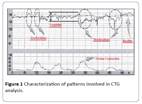
Figure 1: Characterization of patterns involved in CTG analysis.

Three sets of CTG data signals were used in this research to test the proposed algorithm. The first set of 15 CTG data of 30 minutes was collected from the Klinikum Rechts Der Isar, the University Hospital of the Technical University of Munich, and other hospitals in Germany, and this set of 15 CTG data were adjusted (referred as semi-synthetic signals) to include all baseline categories such as normal, bradycardia and tachycardia baseline [22]. The second set consists of 30 CTG signals derived from the first set (referred as synthetic signals). The reason for the use of modified signals semi-synthetic (S1 to S15) and synthetic signals (S16- S45) is to cover all needed features in CTG data such as acceleration, decelerations (late and early deceleration) in some of the selected CTG signals. The third set has 35 clinical data samples (S46- S80) collected from PPUKM (The National University of Malaysia Medical Center) by [23]. The three sets of CTG signals were handed over to two groups of obstetricians, the first group has two experts (Expert 1 and 2), and the second group has three experts (Expert 3, 4 and 5). The obstetricians were asked to estimate the CTG signals parameters: baseline, variability, acceleration, deceleration and their opinion on CTG classification. The obtained computerized results were compared with the estimated results made by the two groups of experts. CTG signals are noisy, containing spiky artifacts, which occur when there are fetal movements or incorrect use of the transducer in the process of monitoring and collecting CTG data signals. The input signal has a missing sample and the graph breakdown to zero (missing beats), the signal condition stage used to remove the breakdown to zero by using if statement through MATLAB source code. In the signal processing stage, the CTG signals are conditioned, by removing spiky artefacts employing a procedure described by [22,24]. This method detects the first stable FHR segments, which are defined as a segment where the difference between five adjacent samples is less than 10 b.p.m. Whenever the difference between five adjacent samples is found to be higher than 25 b.p.m., a linear interpolation is applied between the first of those two signals and the starting of new FHR stable segment. The numbers of interpolated points are used to measure the signal quality [19,21]. The number of values less than 50 b.p.m., is counted to estimate the signal loss. Moving average filter has been chosen in this study to enhance CTG signals and in this section obtaining the ideal value for the filter window size w is. From the figures obtained, the suitable values for the window size are between 30 and 50. In this research paper w=30 for the moving average filter has been chosen by the experts where it gives the best visual interpretation. Values of w beyond 50 distort the shape of CTG data and the data may lose its important features such as variability, accelerations and types and deceleration [21].

Removing spiky signals from the FHR and UC was achieved by using moving average filter, thus eliminating most of the high frequency noise that impairs contraction detection [21,25]. The implementation of the moving average filter to enhance the CTG dataset using MATLAB source code achieved good results, which enabled the experts to interpret the CTG datasets. The implemented algorithm removes unwanted spiky signals and compensates for missing data which affect the experts’ interpretation and extraction of CTG features.

FHR feature extraction

The techniques employed for the FHR and UC features extractions are discussed. Feature extraction is considered to be one of the important steps in CTG signal interpretation, where all the important information related to the fetal condition are extracted, based on which, categorization of the CTG signal is made. Various types of features have been extracted from the FHR signal such as time and frequency domain and morphological features based on EFM guidelines [3]. In this section, a methodology to extract FHR features and CTG classification system based on RCOG guideline [26] are described as shown in Figure 2. All algorithms for feature extraction and classification have been developed and implemented using the MATLAB source code and Excel file. CTG morphological features like baseline, baseline variability, acceleration and deceleration are the most important set of features extracted from the FHR signals. These are the FHR features which are analyzed visually by clinicians in order to estimate and diagnose in everyday practice.

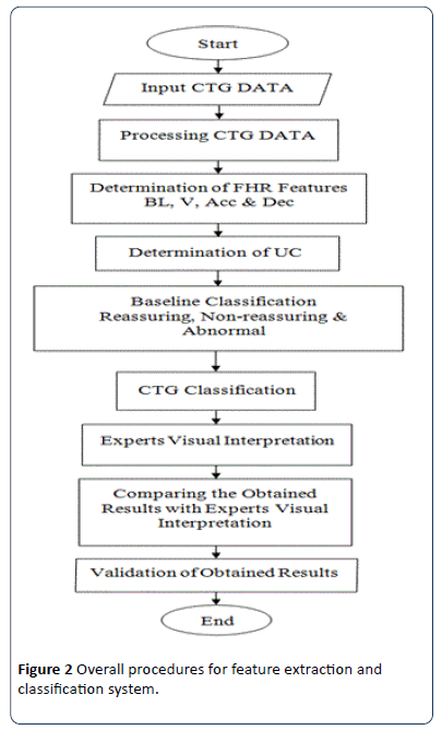
Figure 2: Overall procedures for feature extraction and classification system.

Baseline estimation method

Baseline is the most important feature of the FHR as all other features depend on it. In the field of obstetrics, baseline is an imaginary line that is drawn across the FHR tracing that crosses more points in the FHR signal trace. According to the literature, the computerized estimation of the baseline is a complex process and up to date, there is no consensus on the best methodology that produces the best baseline value [24]. Therefore, a new approach to calculate the baseline is proposed and carefully developed, incorporating some of the points given importance by obstetricians during visual analysis. The procedure employed to calculate real baseline is shown in Figure 3. In this work, a virtual imaginary baseline R is assumed, which is equal to the mean value of the FHR signal of 30 minute segment as in:

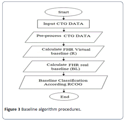
Figure 3: Baseline algorithm procedures.

Where N is the number of samples and y is the CTG signal.

This virtual baseline is the reference to calculate the true baseline BL. This work is based on the MATLAB source code by analyzing the limits of a virtual imaginary baseline of the FHR signal and limiting minimum and maximum values of the input FHR signal to be taken in the evaluation within certain time periods according to the definitions of the RCOG guideline. The first part of the measurement is based on finding the value of R the mean of a 30 minute segment of the FHR signal as explained in Figure 4 [25]. The second part of the measurement is to determine the minimum (L) and maximum (H) limits of the FHR signal as.

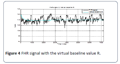
Figure 4: Baseline algorithm procedures.

H = R + a (b.p.m.) ; L = R – a (b.p.m.)

Where a is the value in b.p.m., which is determined by experiments as described in the following paragraphs. The maximum and minimum limits are imposed so that any value above H and below L is neglected. The remaining FHR signal within the limits will be processed in the calculation of the real baseline BL. From experiments using different values of a starting from 1 to 15 b.p.m., added and subtracted from the virtual baseline, the best value of a is selected. The obtained results are compared with the experts’ opinions to find the most accurate result of true baseline; Tables 3 and 4 shows the obtained results of virtual baseline of five selected CTG data.

Table 3 Baseline values for different values of a.

Signals	Values of a
	a=5	a=6	a=7	a=8	a=9	a=10	a=11	a=12	a=13	a=14	a=15
S1	119	122	126	127	129	131	132	135	138	141	143
S4	119	122	124	122	125	125	127	129	129	132	138
S7	133	134	136	135	140	144	145	147	150	149	150
S11	37	139	140	139	141	142	143	143	146	147	150
S15	138	139	139	140	142	144	146	149	151	154	155

Table 4 Comparison of baseline values when a = 8 in table 3 with experts’ estimation.

Interpreted Baseline (b.p.m.)
Signals	Expert 1	Expert 2	Research work	This work
S1	130	130	132	129
S4	120	120-125	125	124
S7	140	140	140	138
S11	140	140	138	141
S15	140	140	140	142

Krupa (2010)

The optimal value of a is 8 b.p.m., which gives the best result and has an accuracy rate of 95% as shown in Figure 5. The accuracy is calculated by comparing calculated real base line value with the average base line of the experts. Figure 6 shows the limits of the FHR signal (H & L) from truncated FHR signal (in red) [24,27].

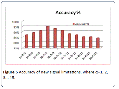
Figure 5: Accuracy of new signal limitations, where a=1, 2, 3... 15.

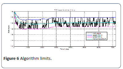
Figure 6: Algorithm limits.

Figure 7 shows the truncated FHR signal without acceleration and deceleration changes. This processed FHR signal may be used to calculate the real baseline according to the RCOG definition [26]. The implemented algorithm calculates the baseline value and classifies whether the BL is reassuring, non-reassuring or abnormal. The decision is made according to the RCOG guideline. The details are shown in Table 1. Figure 8 shows FHR signal with real baseline BL.

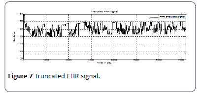
Figure 7:Truncated FHR signal.

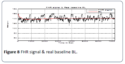
Figure 8:FHR signal & real baseline BL.

Acceleration identification method

The RCOG Guide line defines FHR acceleration as an increase in the FHR by at least 15 b.p.m. from the base line and is sustained at that level or higher for at least 15 seconds as shown in Figure 9. According to the RCOG definition the algorithm identifies all accelerations occurring in a 30 minute FHR pattern recording. The procedure employed to identifies the acceleration is shown in Figure 10.

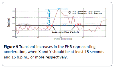
Figure 9:Transient increases in the FHR representing acceleration, when X and Y should be at least 15 seconds and 15 b.p.m., or more respectively.

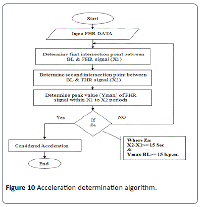
Figure 10:Acceleration determination algorithm.

In this method, the use of a moving average filter smoothens the FHR signal to reduce the number of intersection points between the FHR signal and the BL to the limits without losing the original shape of the signal. In order to calculate intersection points X1 and X2 as shown in Figure 9, the algorithm implemented to detect the intersection points X1 and X2 is based on the match between the (x, y) coordinates of each FHR signal and real baseline points. Another important factor which must be taken into account is the peak of the acceleration period (Ymax) which is the distance in b.p.m. between BL and the highest point of the FHR signal within the period X1 to X2 The implemented algorithm is based on a modified peak detector code built in the MATLAB source code to calculate the maximum value (Ymax) of the FHR signal within a specific time period X1 to X2 in seconds as explained in Figure 10 and Figure 11. According to the RCOG definition of acceleration (Xa and Ya) must be at least 15 b.p.m., and 15 seconds respectively.

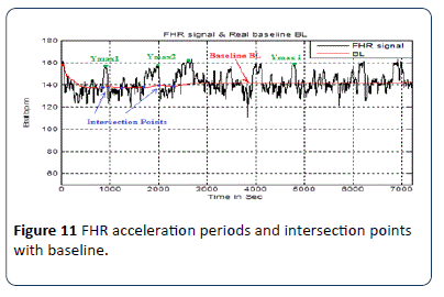
Figure 11: FHR acceleration periods and intersection points with baseline.

Xa = X2 – X1 (Second);

Ya = Ymax – BL(b.p.m.)

The condition (Za) in Figure 10 is true if (Xa is greater or equal to 15 seconds and Ya is greater or equal 15 b.p.m.) In the identification algorithm for the acceleration transient period in the FHR signal, all information data such as the length of (X and Ymax) co-ordinates (position and magnitude) are saved for further CTG classification.

Baseline variability estimation method

The procedure employed to calculate the baseline variability is shown in Figure 12. This part of the algorithm calculates the value of FHR variability V, based on the RCOG guideline definition of baseline variability as shown in Table 1. Figure 13 shows the FHR signal variability in a two minute period. After FHR acceleration occurs and for a period of two minutes, the calculation of baseline variability is based on the calculation of the maximum Ymax and minimum Ymin values of the FHR signal in a two minutes segment after the intersection point between the BL and FHR signal X2. Baseline variability V is calculated as.

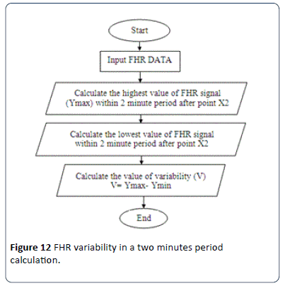
Figure 12: FHR variability in a two minutes period calculation.

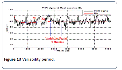
Figure 13: Variability period.

V = Ymax-Ymin

Deceleration identification method

The deceleration pattern is recognized based on the RCOG guideline [26,28,29] where it is defined as, “Transient episodes of slowing of FHR below the baseline level of more than 15 b.p.m. and lasting 15 seconds or more". The procedure employed to identify the decelerations is shown in Figure 14. In addition to the recognition of deceleration patterns, the algorithm distinguishes the deceleration types. The first type is early decelerations; uniform, repetitive, periodic slowing of FHR with the onset early in the contraction and which return to the baseline at the end of the contraction.

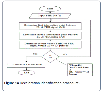
Figure 14: Deceleration identification procedure.

The second type is late decelerations; uniform, repetitive, periodic slowing of FHR with the onset mid to end of the contraction and the nadir more than 20 seconds after the peak of the contraction and ending after the contraction. In the presence of anon-accelerative trace with a baseline variability of less than 5 b.p.m., the definition would include decelerations of less than 15 b.p.m. Figure 15 shows an example of deceleration pattern. In the algorithm X3 and X4 represent the intersection points between the FHR signal and BL. Another factor which must be taken into account is the nadir (the lowest value of FHR signal) of the deceleration period, Ymin. According to the RCOG definition of deceleration, Y and X must be atleast 15 b.p.m. and 15 seconds respectively as.

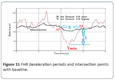
Figure 15: FHR deceleration periods and intersection points with baseline.

Xd = X4 – X3 (Second); Yd = fix(BL - Ymin) (b.p.m.)

The condition (Zd) in Figure 14 is true if (Xd and Yd) are at least 15 second or more and 15 b.p.m., or more respectively. All information about deceleration in the FHR signal, such as number of decelerations and types of decelerations (Early or Late) are extracted and saved for further classification of CTG based on the RCOG guideline as shown in Table 1.

Uterine contraction estimation method

The other feature that must be taken into account is uterine contractions (UC) as shown in Figure 16. The UC calculation algorithm is used to find the number of UC occurring in a CTG pattern and calculates the value of UCmax which represents the reference point for calculating any type of deceleration, whether it be late or early. The information about UC in the CTG signal such as the number of UC and values of UCmax are extracted and saved for further classification of the CTG based on the RCOG guideline.

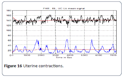
Figure 16: Uterine contractions.

The procedure employed to calculate the types of decelerations is shown in Figure 17. To calculate the type of deceleration, whether it is late or early, the value of the time tYmin for deceleration Ymin and the value of time for uterine contraction tUCmax of UCmax must be obtained first as shown in Figure 18 (a and b).

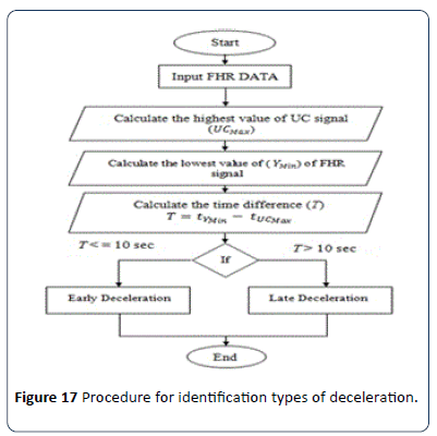
Figure 17:Procedure for identification types of deceleration.

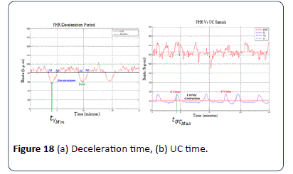
Figure 18: (a) Deceleration time, (b) UC time.

Figure 19 shows the time difference T in seconds between the deceleration and UC in the CTG signal. T is the factor for estimating the type of deceleration, whether it is early or late according to the RCOG guideline. If T is greater than 10 seconds, then the deceleration is late deceleration and if T is less than 10 seconds, the deceleration type is early deceleration where.

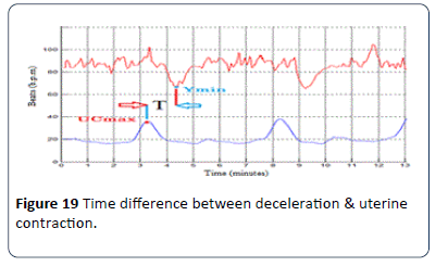
Figure 19: Time difference between deceleration & uterine contraction.

T = tYmin - tUCmax

CTG classification algorithms

The implemented classification algorithm imports the FHR features (baseline, baseline variability, acceleration and type of deceleration) and UC information extracted previously into the MATLAB rule based functions. According to the information provided in Table 2 combined score of the FHR signal is estimated. There are three conditions for CTG trace pattern classification, condition (A) if all CTG features fall in the reassuring category, condition (B) if all CTG features fall in the Non-reassuring category and condition (C) if CTG features fall the two or more of Non-reassuring category or one in abnormal category. All procedure steps are illustrated in Figure 20. The proposed algorithm for the CTG Dataset classification is based on MATLAB source code. The classification algorithm implemented based on MATLAB source code relies on the RCOG guideline classification sets as in Tables 1 and 2. The algorithm classified the input data (baseline, baseline variability, acceleration and deceleration) in the following sets: If all inputs are in the reassuring category, then the CTG classification is "Normal"; however, if one of the inputs is in the Non-reassuring category and the remaining inputs are in the reassuring category, then the CTG type is "Suspicious", else, the CTG type is "Pathological". To ensure the validity of the implemented classification algorithm, the second algorithm was utilized to verify the results obtained.

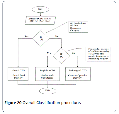
Figure 20: Overall Classification procedure.

Validation techniques

Statistics is defined as a tool for creating new understanding from a set of numbers. It has become an integral part of biomedical research because of its ability to deal with data collection, presentation, analysis and interpretation for the purpose of drawing a conclusion. Statistics have been used in this study at various levels, ranging from data representation to validation. There are many statistical methods used to verify the validity of the obtained classification results, which rely on a comparison between the results and the interpretation of experts in the field of biomedical signal processing. In this work kappa statistics has been implemented.Generally known as Cohen's kappa coefficient [25,26], it is a statistical measure to evaluate the inter-rater agreement between two classifications and claims to eliminate any agreement arrived by chance. The kappa value can be estimated as.

where P(a) is the relative observed agreement and P(e) is the hypothetical probability of chance agreement, which are estimated from the relationship in Table 5. The interpretation of K value is done as shown in Table 5.

Table 5 Interpretation of k value.

Value of k	Strength of agreement
<0.20	Poor
0.21-0.40	Fair
0.41-0.60	Moderate
0.61-0.80	Good
0.81-1.00	Very good

Results and Discussion

In this section the results obtained from the morphological feature extraction algorithms developed using conventional programming techniques and the classification system based on RCOG guideline are discussed. The results obtained from the algorithms are compared with the visual interpretation results of five experienced Obstetricians as it is considered a gold standard in CTG interpretation. Baseline is the fundamental feature of FHR signal and other features rely completely on it, hence its algorithm validation is first described. The effectiveness of the feature extraction methods is discussed. Towards the end of the chapter the performance of the classification system is evaluated.

Signal enhancement results

Moving average filter has been chosen to enhance CTG signals and in this section obtaining the ideal value for the filter window size w is obtained as in Figure 21. From the figures obtained, the suitable values for the window size are between 30 and 50. In this research w=30 for the moving average filter has been chosen by the experts where it gives the best visual interpretation. Values of w beyond 50 distort the shape of CTG data and the data may lose its important features such as variability, accelerations and types and deceleration [22,29]. Removing spiky signals from the FHR and UC wasachieved by using moving average filter, thus eliminating most of the high frequency noise that impairs contraction detection [18,22,30]. The implementation of the moving average filter to enhance the CTG dataset using MATLAB source code achieved good results, which enabled the experts to interpret the CTG datasets. The implemented algorithm removes unwanted spiky signals and compensates for missing data which affect the experts’ interpretation and extraction of CTG features. Figures 22a and b show a sample signal of the CTG data before and after removing unwanted signals (noise).

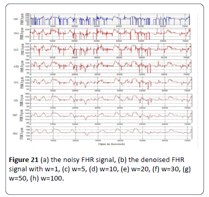
Figure 21: (a) the noisy FHR signal, (b) the denoised FHR signal with w=1, (c) w=5, (d) w=10, (e) w=20, (f) w=30, (g) w=50, (h) w=100.

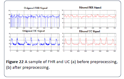
Figure 22: A sample of FHR and UC (a) before preprocessing, (b) after preprocessing.

Baseline estimation results

For first set of signals, baseline is estimated by using the proposed algorithm. The results obtained from the algorithm are stored in excel file for further analysis. Results obtained for first signal set are provided in Figure 23. The baseline results shows a slight difference between the obtained results and the results of the experts and researcher. The output results are all different within (±2) b.p.m., and almost similar to the experts estimated results.The second set of data signals S16-S45 are used to test the algorithm. The same sample signals were handed over to three different obstetricians (Expert 3, 4 and 5). Obstetricians were asked to estimate the FHR samples baseline; the computerized results are compared with the estimated results made by the three experts as shown in Figure 24. The output results are all within (±3) b.p.m., and almost similar to the experts estimated results, except signal S20 and S25, where the two signals are irregular CTG signals.

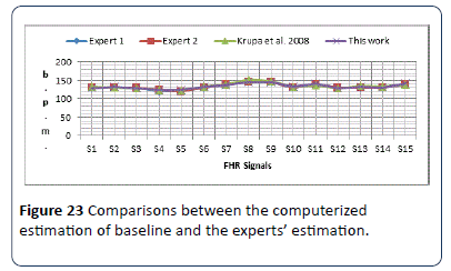
Figure 23: Comparisons between the computerized estimation of baseline and the experts’ estimation.

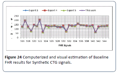
Figure 24: Computerized and visual estimation of Baseline FHR results for Synthetic CTG signals.

The obtained results show the baseline of the 30 CTG signals were all in the reassuring category (RCOG 2003) except signals (S17, S19, S22, S23 and S31) were considered non-reassuring and S35 where considered in abnormal category. The third set of data which is the clinical signals was then used to test the algorithm. The same sample signals were handed over to (Experts 3, 4 and 5). Obstetricians were asked to estimate the FHR samples baseline; the computerized results are compared with the estimated results made by the three experts as shown in Figure 25. The output results are almost similar to the experts estimated results are all within (±4) b.p.m., except signal S54 and S66.

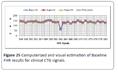
Figure 25: Computerized and visual estimation of Baseline FHR results for clinical CTG signals.

Variability estimation results

The baseline variability computerized results are compared with the estimated results made by three experts on two sets of CTG data with the first set being S16-S45 and the results shown in Figure 26.

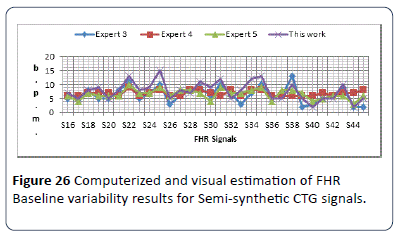
Figure 26: Computerized and visual estimation of FHR Baseline variability results for Semi-synthetic CTG signals.

The output results are all within (±5) b.p.m., and almost similar to the experts estimated results except signal S25, there is a difference between the presentation of each expert estimated results due to the difference in their hospitals system guidelines. The obtained results show the baseline variability of the 30 CTG signals were all in reassuring category, except signals S17, S20, S26 and S32 were considered nonreassuring. The test on the third set S46-S80 has results as shown in Figure 27. The output results are all within (±5) b.p.m., difference and almost similar to the experts estimated results except the estimation of the second expert which gives higher range of variability estimation. All signals are in reassuring category except signals S37, S40, S41, S43, S45, S47, S49, S50, S51, S53, S59, S61, S63, S65, S66 and S68 are nonreassuring. There is a difference between the presentations of each expert estimated results due to the difference in their hospitals system guidelines.

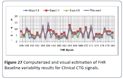
Figure 27: Computerized and visual estimation of FHR Baseline variability results for Clinical CTG signals.

Acceleration identification results

The identification algorithm has been explained carefully in the previous chapter, and in this section the output results for detecting the number of accelerations are given. The algorithm calculates number of acceleration occurring in 30 minute CTG pattern. Figure 28 shows the output results for 30 CTG samples synthetic signals (S16-S45). The obtained results in Figure 28 shows the worst difference of (±4) compared with the three expert estimated results. In this algorithm and according to RCOG guideline, the most important aspect in acceleration calculation is the presence or absence of acceleration and the number of acceleration is not taken into account. The clinical signals (S46-S80) are also used in the algorithm to estimate the number of accelerations as shown in Figure 29. The obtained results in the table show the worst difference of (±6) compared with the three expert estimated results. From Figure 28 and 29, in general all the output results are similar to the three experts estimated number of accelerations with difference of (1 or ±2) number of accelerations. Due to the difference in experts experience and adopted guidelines, there are some exceptions which result in the worst cases.

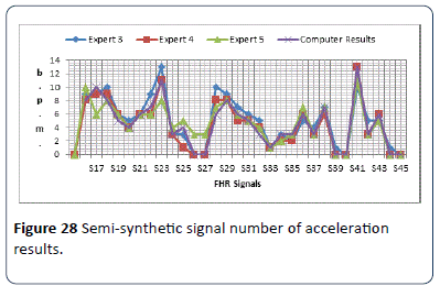
Figure 28: Semi-synthetic signal number of acceleration results.

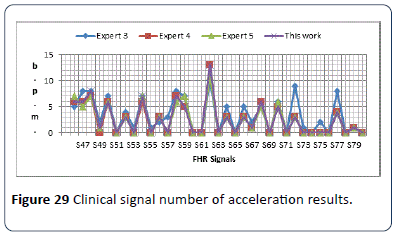
Figure 29: Clinical signal number of acceleration results.

Deceleration identification results

The identification algorithm has been explained carefully in the previous chapter, and in this section output results for number and types of decelerations are given. The algorithm calculates number of decelerations occurring in 30 minute CTG pattern, and identify types of decelerations whether its early (E) or late (L). Figure 30 shows the output results for S16-S45. The second set of data is (S46-S80) is used in the algorithm to estimate the number and types of decelerations as shown in Figure 31. From the results obtained in Figures 30 and 31, all the output results are similar to the experts estimated number and type of decelerations. The results in both Figure 30 and 31 shows the same type of deceleration (Late & Early).

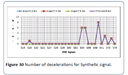
Figure 30: Number of decelerations for Synthetic signal.

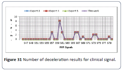
Figure 31: Number of deceleration results for clinical signal.

CTG classification results

The classification of CTG signal is implemented using fuzzy logic tool box built in MATLAB. Figure 32 illustrates the classification obtained results for S16-S45 synthetic CTG signals, where N is normal, S is suspicious and P is pathological.

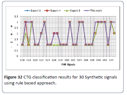
Figure 32: CTG classification results for 30 Synthetic signals using rule based approach.

The obtained results in Figure 33 show no significant difference between the experts’ visual interpretation and the algorithm classification results. Figure 32 illustrates the classification obtained results for 35 clinical signals compared with three obstetricians (expert) opinion. The obtained results in Figures 32 and 33 show a slight difference in classification of CTG signals between computer results and the three experts, due to the differences in experts visual interpretation experience and hospitals adopted guidelines.

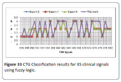
Figure 33: CTG Classification results for 35 clinical signals using fuzzy logic.

Statistical analysis of classified CTG data

The final step in this research is the statistical validation between obtained CTG classification results and the three obstetricians visual interpretation based on Kappas core. The obtained results show a promising kappa value between the implemented algorithm and the three experts visual interpretation. Table 6 shows the statistical agreement.

Table 6 Degree of agreement of the classified results.

Table Numbers	Agreement between Obtained results and Experts	Kappa value	Type of Agreement
4.1	Expert1	0.916	Almost perfect agreement
	Expert 2	0.916	Almost perfect agreement
	Expert 3	0.651	Substantial
4.11	Expert1	0.668	Substantial
	Expert 2	0.587	Moderate
	Expert 3	0.63	Substantial
4.12	Expert1	0.916	Almost perfect agreement
	Expert 2	0.916	Almost perfect agreement
	Expert 3	0.651	Substantial
4.13	Expert1	0.668	Substantial
	Expert 2	0.587	Moderate
	Expert 3	0.63	Substantial

Conclusion

In this paper different techniques for FHR features extraction and classification have been developed along with a new signal enhancement method for CTG signals. Firstly, in the developed method morphological features were extracted and classified based on RCOG guideline. The use of RCOG guideline in the interpretation of FHR features brought in a systematic and organized approach to CTG classification. Furthermore, the effectiveness of this system evaluated by comparing the results with those of experts visual interpretation using MATLAB source code showed satisfactory levels of performance. It also proved that no significant difference exists between the method and experts visual interpretation, for the set of synthetic CTG signals and a slight difference for the clinical CTG signals used for validation. Secondly, the new CTG signals enhancement technique has been developed involving an algorithm for compensating missing value segments and removing high frequency noise. The effectiveness of the method is measured with the help of a comparative study on various signal enhancement methods employed in the past and ratings obtained for the resulting signals, based on the visual quality, from three obstetricians.

Finally, a method has been developed for the FHR feature extraction and classification. The method involves extraction of FHR features from the decomposed components of the FHR signals and their classification using fuzzy logic tool box built in MATLAB. The effectiveness of this method was evaluated by determining the accuracy of prediction using the visual classification results from three obstetricians as references. In addition, statistical methods were employed to confirm the accuracy of classification based on the visual interpretation of three obstetricians, kappa values of 0.916, 0.916 and 0.651 and 0.668, 0.587 and 0.630 for the synthetic and clinical CTG signals respectively.

Even though obtained results proved the viability of the techniques developed an extensive validation on a larger data set is required, in order for those to be employed in everyday clinical practice.

17436

References

1. Philip P, Taillard J, Léger D, Diefenbach K, Akerstedt T, et al. (2002) Work and rest sleep schedules of 227 European truck drivers. Sleep Med 3: 507-511.
2. Va´rady P, Wildt L, Benyo´ Z, Hein A (2003) An advanced method in fetal phonocardiography. Comput Methods Programs Biomed 71: 283-296.
3. Fausta O, Acharyab UR, Jianguo M, Minb LC, Tamurad T (2012) Compressed sampling for heart rate monitoring. Comput Methods Programs Biomed 108: 1191-1198.
4. Peters M, Crowe J, Piéri J, Quartero H, Hayes-Gill B, et al. (2001) Shakespeare, Monitoring the fetalheart  non-invasively: A review of methods. J Perinat Med 29: 408-416.
5. Kovács F, Horváth C, Balogh AT, Hosszú G (2011)Fetal phonocardiography-Past and future possibilities.Comput Methods Programs Biomed 104: 19-25.
6. Royal College of Obstetricians and Gynaecologists (RCOG) (2003) The use of electronic fetal monitoring. Evidence based guideline, RCOG Press, London, United Kingdom.
7. Dawes GS, Moulden M, Redman CW(1996) Improvements in computerized fetal heart rate analysis antepartum. J Perinatal Med 24: 25-36.
8. Warrick PA, Kearney RE, Precup D, Hamilton EF (2006) System-Identification noise suppression for intra-partum cardiotocography to discriminate normal and hypoxic fetuses.ComputCardiol 33: 937-940.
9. Mika P,Tarvainena B, Niskanena JP, Lipponena JA, Ranta-ahoa PO, et al. (2013)Kubios HRV – Heart rate variability analysis software.Comput Methods Programs Biomed 113: 210-220.
10. Declan D (2005) Midwives’ visual interpretation of intrapartumcardiotocographs: intra- and inter-observer agreement.J AdvNurs 52: 133-141.
11. Maria C,Nunes da AM (2011) Development and evaluation of a combination of computer analysis of cardiotocografy and electrocardiography for intrapartumfetal monitoring. PhD Thesis, University do Porto, Portugal.
12. Zuckerwar AJ, Pretlow RA, Stoughton JW, Baker DA (1993) Development of a piezopolimer pressure sensor for fetal heart rate monitor, IEEE Trans Biomed Eng 40: 963-969.
13. Talbert DG, Davies WL, Johnson F, Abraham N, Colley N, et al. (1986) Wide bandwidth fetal phonocardiography using a sensor matched to the compliance of the mother’s abdominal wall, IEEE Trans Biomed Eng 33: 175-181.
14. Kovács F, Török M, Habermajer I (2000) A rule-based phonocardiographic method for long-term fetal heart rate monitoring, IEEE Trans Biomed Eng 47: 124-130.
15. Georgoulas G, Stylios CD,Groumpos PP (2005) Classification of fetal heart rate using scale dependent features and support vector machines.Proceedings of 16th IFAC World Congress.
16. Georgoulas G, Stylios CD,Groumpos PP (2006) Predicting the risk of metabolic acidosis for newborns based on fetal heart rate signal classification using support vector machines. IEEE T Bio-Med Eng53: 875-884.
17. Struzik ZR,Wijngaarden WJ (2001) Cumulative effective holder exponent based indicator for real time fetal heartbeat analysis during labour. Report INS-R0110.
18. Freeman RK, Garite TJ,Nageotte MP (2003)Fetal heart rate monitoring.(3rd edtn) Lippincott Williams and Wilkins, Philadelphia.
19. Guijarro-Berdinas B, Alonso-Betazos A,Fontenla-Romero O (2002) Intelligent analysis and pattern recognition in cardiotocographic signals using a tightly coupled hybrid system. ArtifIntell Med 136: 1-27.
20. Bernardes J, Moura C, Sa JPM, Pereira-Leite L (1991) The Porto system for automated cardiotocographic signal analysis. J Perinat Med 19: 61-65.
21. Ayres-de-Campo D, Bernardes J, Garrido A, De Sa JPM, Pereira-Leite L (2000) SisPorto 2.0: a program for automated analysis of cardiotocograms. J MaternFetal Med 9: 311-318.
22. Krupa BN, Mohd AMA, Zahedi E, Shuhaila A,Fauziah MH (2011) Antepartum fetal heart rate feature extraction and classification using empirical mode decomposition and support vector machine. BioMedEng 10: 6-20.
23. Krupa BN (2010) Perinatal cardiotocography signal analysis and classification. PhD Thesis, University Kebangsaan, Malaysia.
24. Shahad N, Mohd Ali MA, ZaidanAA, Zaidan BB,Najah H(2010) A novel cardiotocographyfetal heart rate baseline estimation algorithm. Sci Res Essays 5: 4002-4010.
25. Ayres-de-Campos, Ugwumadu A, Banfield P, Lynch P, Amin P, et al. (2010) A randomised clinical trial of intrapartumfetal monitoring with computer analysis and alerts versus previously available monitoring. BMC Pregnancy Childbirth 10:71.
26. Royal College of Obstetricians and Gynaecologists (RCOG)(2003) The use of electronic fetal monitoring. Evidence based guideline. RCOG Press, London, United Kingdom.
27. Mamdani EH,Assilian S (1975) An experiment in linguistic synthesis with a fuzzy logic controller.Int J Man-Mach Stud 7: 1-13.
28. Christian W, Pfirrmann M, Metzdorf A, Zanetti M, Hodler J,et al. (2001) Magnetic resonance classification of lumbar intervertebral disc degeneration. SPINE 26: 1873-1878.
29. Weibei D,Ren Y, Wu Q,Ruan S,Chen Y, et al. (2007) Fuzzy kappa for the agreement measure of fuzzy classifications. International Conference on Intelligent Computing 70: 726-734.
30. Shahad N, Mohd Ali MA,Najah H(2011) Computerized algorithm for fetal heart rate baseline and baseline variability estimation based on distance between signal average and α value. Int J Pharmacol 7: 228-237.